
Afterglow Astrophotography
Funded by a $3M Department of Defense Education grant, we have been adding astrophotography capabilities to our web-based Afterglow software. The goal is to make astrophotography easier, so it can be incorporated into survey-level courses. We aim to achieve 85% of the quality of an APOD, but with only 15% of the learning curve/buttons to press.
This page is a blog of my own efforts, with latest entries at the top. The descriptions will be fairly technical, to assist future students with their own astrophotography adventures.

11/29/2022
Messier 42, the Orion Nebula (Part II)
Check out my post below for the main processing (A, below). Here, I’m again playing with lightening and clarity adjustments, post-Afterglow processing. In B, I increased the clarity 50%. Again, I was very tempted to go with 100%, but (after the fact) realized that it looked a bit over-processed, and dialed it back down. Thing to keep in mind is with increased clarity comes increased noise — it’s not deconvolution, it’s just sharpening.
In C, I increased the lightening 50%. And in D, I instead decreased it 100%. Neither of these are good final images. C blows out the middle, but reveals greater detail in the outskirts. In D, the outskirts are lost, but you get a better view of the Trapezium, and the inner star cluster.
Going with B as my final image, but C and D are exciting complements.


11/29/2022
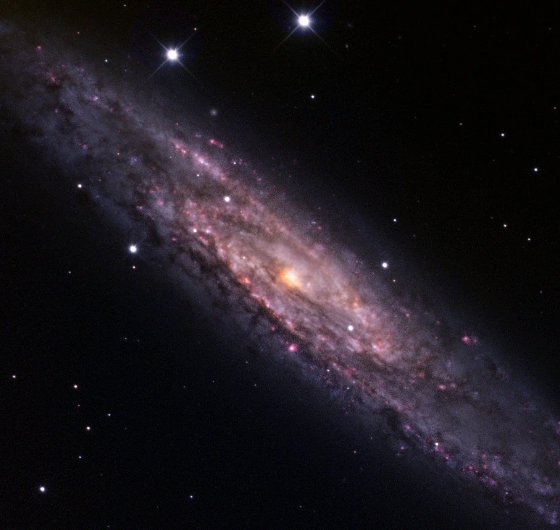
NGC 253, the Sculptor Galaxy (Part II)
Check out my post below for the main reduction (A, below). Here I’m playing with basic lightening and clarity adjustments, after the fact. Just using Window’s basic picture viewer/editor — nothing fancy. In B, I darkened the image 50%. In C, I increase the clarity 50%. And in D, I instead increased it 100%.
I’m assuming that “clarity” is just wavelength sharpening. When I do wavelet sharpening in Afterglow, (1) it’s not reversible, and (2) it does a terrible job with saturation bleeds. This, however, is reversible, and it seems to navigate bleeds, so there must be something extra here. Going to build this in as a final step for my student-level guide.
However, I noticed that it doesn’t improve every image. And it’s easy to overdo it. In particular, D looks over-processed. Many images of Sculptor look this way — and I can understand the temptation. Will encourage my students to use a little self-control here.
Going with C as my final image.


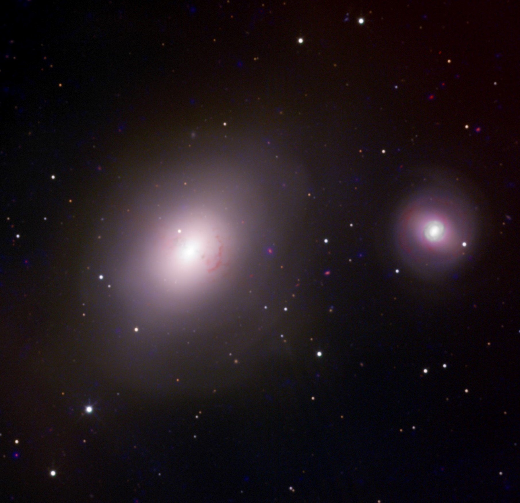
This is NGC 1316 (also known as Fornax A) and its smaller companion, NGC 1317. 1316 is a lenticular galaxy — something between an elliptical and a spiral. 1317 is a barred spiral.
First, I collected 6.6 hours of LRGB data with Skynet's 16-inch diameter PROMPT-6 telescope in Chile, and combined it, correcting for the reddening effects of dust.
Then, I supplemented it with mid-infrared data from NASA's Spitzer spacecraft. Here pinker colors highlight warm dust (about 300 Kelvin) and bluer colors highlight cool dust (about 100 Kelvin).
Also notice all the pink/purple/blue background points. Each one is a galaxy like these two, with its own warm/cool dust, just much farther way.
For the details: https://www.danreichart.com/afterglow-astrophotography/#ngc1316
11/13/2022
NGC 1316 and 1317, in the Fornax Cluster
I’ve been imaging a lot of spiral galaxies, so I decided to try something more complicated. On the left, we have NGC 1316, known in the radio as Fornax A. It’s a lenticular galaxy, which is something between a spiral and an elliptical — no spiral arms, not much star formation, but possibly a lot of dust. It appears to be the product of one or more recent, large galaxy mergers. Gas disrupted in these mergers has been feeding the accretion disk about its central, supermassive black hole. This disk then creates massive, radio-emitting outflows, called jets, making Fornax A the 4th brightest source in the radio sky (at 1.4 GHz).
On the right, we have NGC 1317, a barred spiral galaxy that may or may not be interacting with NGC 1316 (they might be at the same distance, or it might be a projection effect).
For this complicated pair of targets, I collected 1.5 hours in each of R, V, B, and H-alpha, and 2.1 hours in Lum, using our 16-inch diameter PROMPT-6 telescope at Cerro Tololo Inter-American Observatory in Chile.
First I combined the R, V, and B layers, correcting only for line-of-sight dust in the Milky Way (E(B-V) = 0.019 mag; A, below). Next, I had to decide how much dust to correct for in the galaxies, noting that the galaxy on the right might have more dust than the galaxy on the left — and I can remove only a single amount. In B, I correct to a depth where 25% of the blue light is removed with respect to the green light, making both galaxies bluer. In C, I apply my “cake” method, in which I correct to a depth where 50% of the blue light is removed with respect to the green light, but then combine this with B using the lighten blend mode. This makes the galaxies even bluer, but without over-correcting the generally redder field stars.
Which should I use? If the galaxy on the left were an elliptical, devoid of dust, A would be the best choice for it. For the spiral galaxy on the right, C is probably best — my “cake” method usually does a pretty good job on spirals. Lenticulars are something in-between, so maybe B or C would be best for the galaxy on the left, depending on how much dust is in there. I have to pick one, so I’m going with C.
Next, I had to decide what to do with my H-alpha layer. I hate throwing data away, but this layer really didn’t add anything — no star-forming regions, just a diffuse glow across each of the galaxies. Trying to incorporate it just changed the color of the galaxies, and increased the image’s color noise. In the end, I decided to ditch it.
So, that’s my visible-light picture. But there’s always more to the story in the infrared. NASA’s Spitzer spacecraft mosaiced this field at 8 and 24 microns. At these wavelengths, you’re mostly imaging warm (about 300 K) and cooler (about 100 K) dust, and since both of these galaxies are dusty, that should be interesting. I added the warm dust layer in D, using the “heat” color palette, and the cool dust layer in E, using the “cool” color palette. (In the end, I placed a bit more emphasis on the “cool” layer than the “heat” layer, but this was mostly an aesthetic choice.)
Notice how the dust lanes in both galaxies now glow. Also notice how many of the background points now glow pink/purple/blue. These are all galaxies too, with their own star formation heating dust, which then re-emits this energy in the mid-infrared. This dust is warmer in the pinker galaxies, and cooler in the bluer galaxies.
Lastly, I cropped it a bit in F.
Technical note: To avoid saturating the centers of the galaxies, which are very bright in the mid-infrared, and especially the center of the spiral galaxy where there is interesting detail, I put the luminance layer above all of the layers, instead of just above the RVB layers.


I've mostly caught up on my other work, so back to testing our new (and still developing!) astrophotography software (Afterglow Access), for students.
This is (of course!) the Great Nebula in Orion, which is so bright you can see it with the naked eye. For this one, I used our 32-inch diameter PROMPT-7 telescope in Chile, and acquired 16 minutes in LRGB + 1.5 hours in narrowband hydrogen (pink) and oxygen (blue-green) filters.
To this I added 5.8 micron mid-infrared data from NASA's Spitzer spacecraft (orange), which shows where these stars are heating the surrounding, dusty clouds from which they formed, and 2.2 micron near-infrared data from the ground-based 2MASS survey (blue). These also reveal stars that we otherwise wouldn't be able to see, hidden by this dust at visible wavelengths, but not in the infrared.
For the details: https://www.danreichart.com/afterglow-astrophotography/#messier42.
11/12/2022
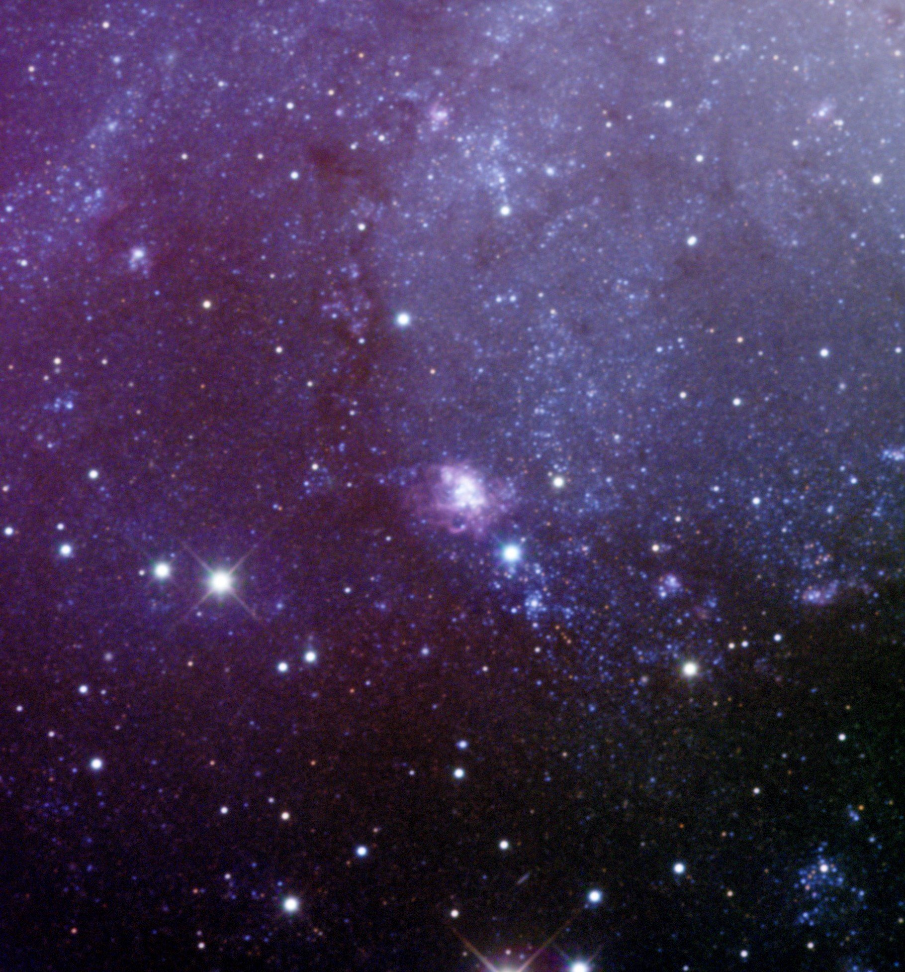
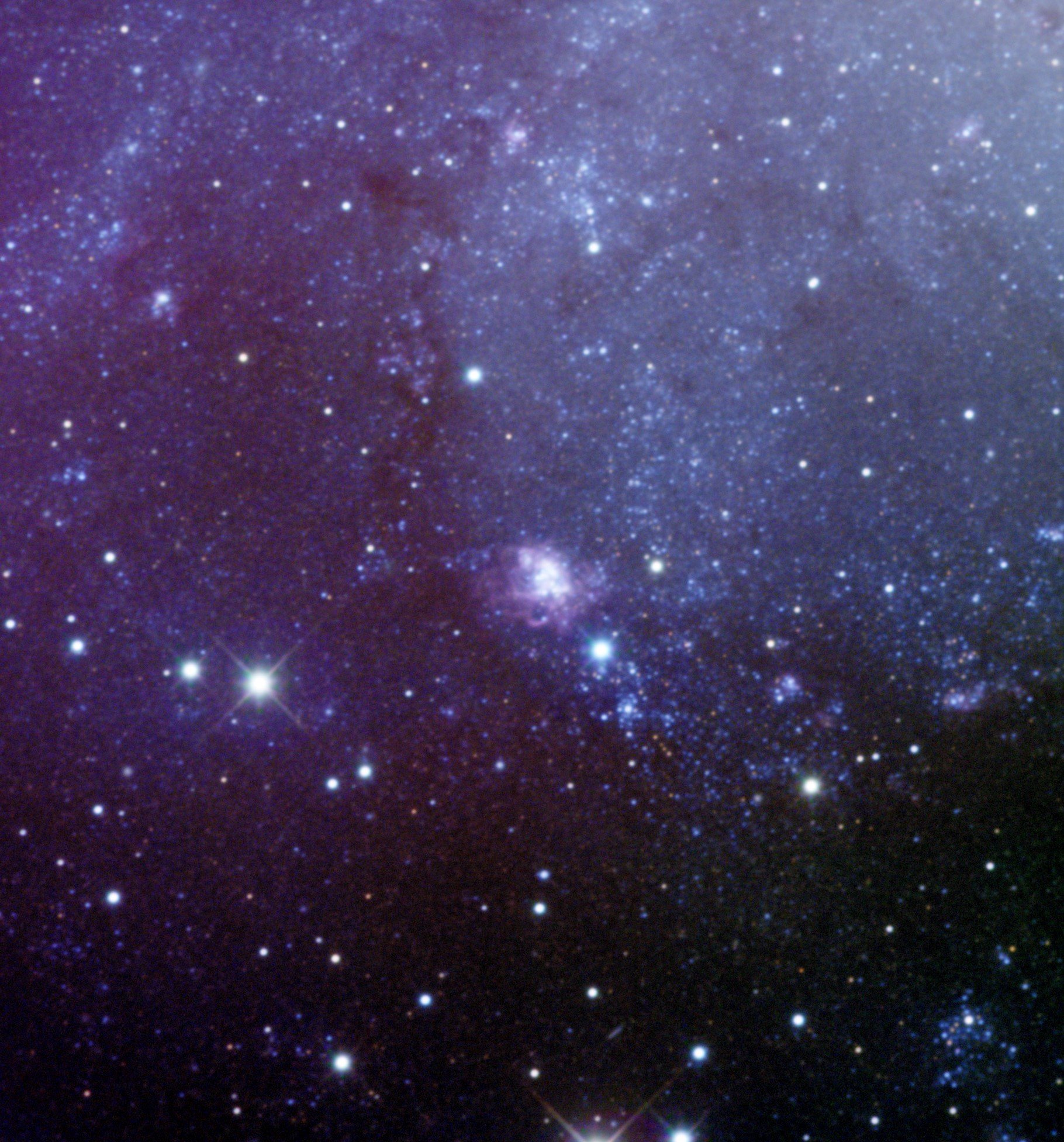
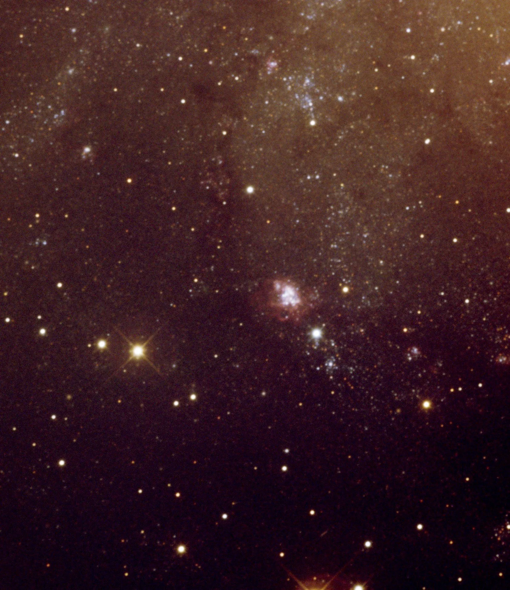
Messier 42, the Orion Nebula
Also known as the Great Nebula in Orion, you can see this one with the naked eye — it’s the middle “star” in Orion’s sword. Had to give it a go!
For this one, I used our 32-inch diameter PROMPT-7 telescope at Cerro Tololo Inter-American Observatory in Chile. It’s so bright, I collected only 2.7 min in Red, 4.5 min in Green, 6 min in Blue, and 2.7 min in Lum. But I also collected 45 min in each of H-alpha, OIII, and SII. The SII wasn’t high enough signal-to-noise to use, but the rest turned out great, and all collected in a single night.
You can see the Red/Green/Blue combination in A, below. It gets the stars just fine, but its capture of the nebulosity is a little ho-hum. So I then boosted this with my H-alpha and OIII layers, coloring them our custom Balmer and OIII colors (B).
Nice, except its starting to blow out the center. So then I applied my broadband luminance filter (C). Normally, I would apply this after my RGB layers but before my narrowband layers. But despite having only 2.6 min of this, and despite M42 being primarily a narrowband target, it has great signal-to-noise, so why not! It doesn’t appear to degrade the signal-to-noise of the nebulosity, but it also tamps it down at the center, letting the bright stars there shine through.
This is an awesome — but very typical — picture of Orion. So let’s jazz it up with some infrared data. In D, I add on a 5.8 micron, mid-infrared mosaic from NASA’s Spitzer spacecraft. I would have preferred using Spitzer’s 8 or 24 micron bands, to focus on just the warm, star-heated dust, but these had too many defects (as did lower-resolution data from NASA’s WISE spacecraft — this target is just too bright!) At 5.8 microns, you get both warm dust and stars (but also higher resolution!)
I colored this layer with the “heat” color palette. To balance out these new, previously dust-hidden — but very orange — stars, I added on 2.2 micron (K-band), near-infrared data from the ground-based 2MASS survey (E). I colored this with the “cool” color palette, but used the lighten blend mode to avoid blowing out the center again. (The lighten blend mode doesn’t work well with the heat color palette, so I took a bit of a hit in the center with that layer.)
Lastly, I cropped/reframed it (F).
So what’s going on here? These stars are on the edge of a very large, dark, dusty cloud (it extends far off the image, toward the left, top left, and top). The bright stars in the center (the “Trapezium”), as well as another bright star near the top of the image, are ionizing surrounding gas. This gas recombines, with hydrogen and twice-ionized oxygen (OIII) emitting bright lines in the visible part of the spectrum (pink and blue-green, respectively). (The Trapezium’s hot enough to produce both, but the single star near the top of the image is a bit too cool to produce OIII.)
This hot, ionized gas is expanding, pushing against the cloud from which these stars formed. Dust in these clouds is also being heated by these stars, and re-emitting in the mid-infrared (orange). Also, stars, hidden at visible wavelengths by this dust, shine through in the mid- (orange) and near- (blue) infrared, giving us some additional orange/pink/purple/blue stars.


10/3/2022
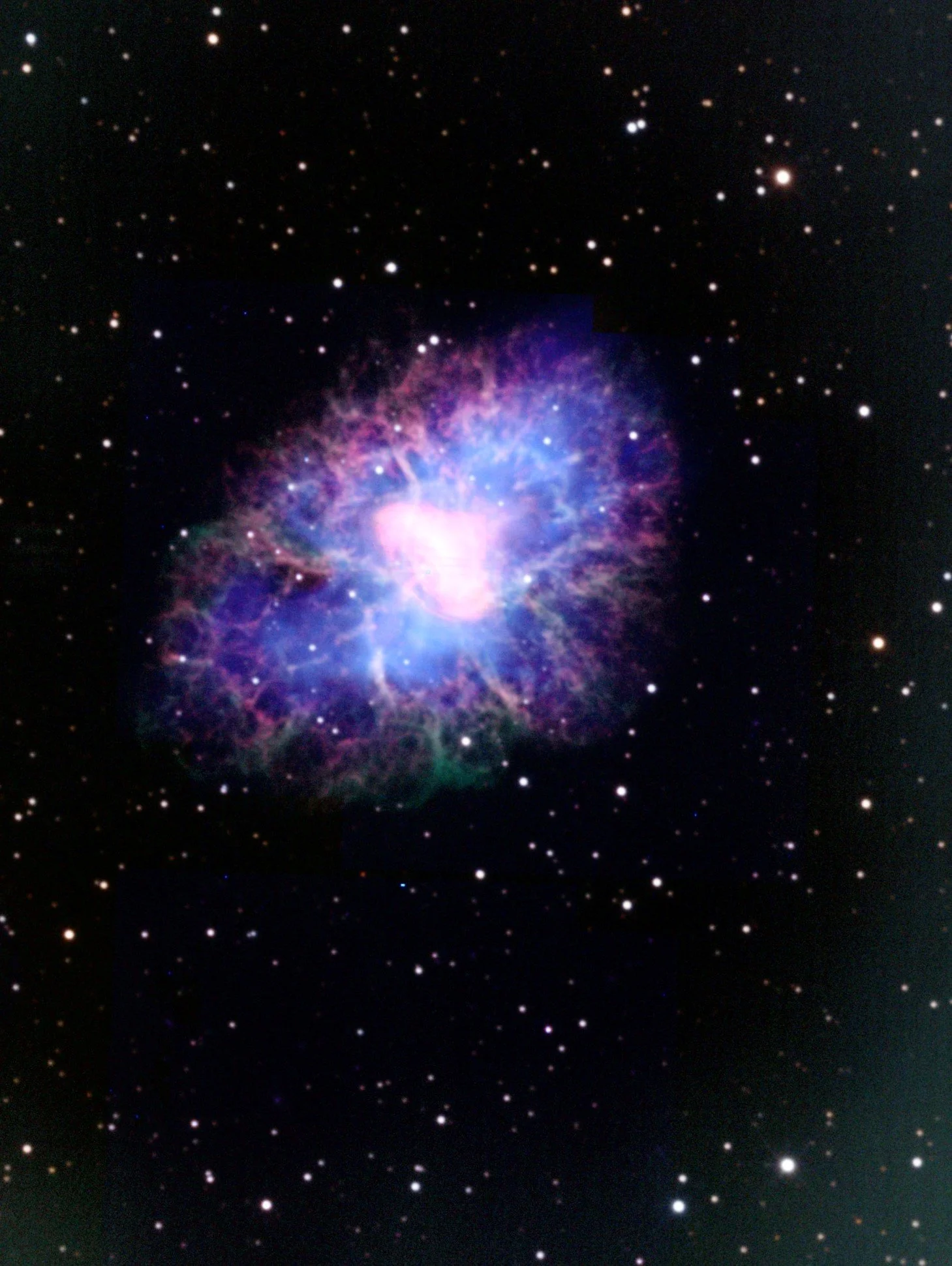
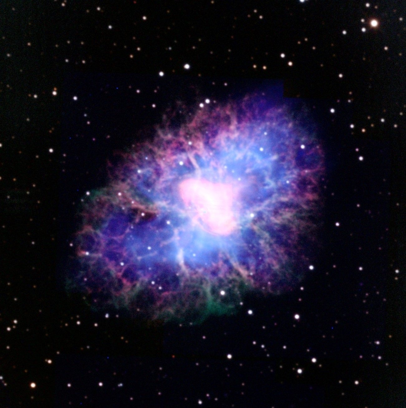
Messier 1, the Crab Nebula
I did a planetary nebula below (the Helix). Now it’s time for massive star death — supernova remnants. I’ve come to learn that there’s the Crab, and then there’s everything else. The Crab is young and compact — easily fits within our telescopes’ FOV. Everything else (that we can readily detect) is old, big, and wispy. I’ll try one of them later.
These are all narrowband targets, though I still collected LRGB for the stars. This time, I got 19 min of Lum, 14 min of R, 20 min of V, and 26 min of B. But then I got 135 min of H-alpha and (drumroll please…) 336 min of OIII. I really didn’t need that much H-alpha and especially OIII. However, I had a dark-subtraction problem that I was (incorrectly) trying to fix by collecting more data to beat down the noise. (Skynet stopped collecting darks after the first night, but kept auto-reducing with that same, increasingly inaccurate, master dark. Didn’t figure it out until it was all done, over a week later…no fixing it now!)
You can see the LRGB combination in A (below), which I’ve corrected for E(B-V) = 0.52 mag of reddening by intervening dust. You can see the H-alpha narrowband emission surrounding the remnant. It’s white middle is due to synchrotron emission, from magnetic fields. This component can be imaged at invisible wavelengths as well, from radio through X-ray (see below).
In B, I dim the LRGB layer way down — enough that when I add the narrowband layers (see below), they dominate the nebular emission, but not so much that they dominate and (significantly) recolor the stars.
I add my H-alpha layer on in C, and my OIII layer on in D. I really had to stretch/brighten the OIII layer, so it could compete with the H-alpha layer. This is also revealing my dark-subtraction problem, which I partially hid by raising the OIII layer’s background level. Here, I’m using our natural “Balmer” and “OIII” colors and the screen blend mode.
Then for the non-visible components: I layered on 3.6-micron, near-infrared data from NASA’s Spitzer observatory (E and F), to highlight the synchrotron emission, and X-ray data from NASA’s Chandra observatory (G and H), to highlight the pulsar wind nebula in particular — thanks Jonathan Keohane!
Lastly, I crop out the rest of my dark-subtraction problem, and the most significant 3.6-micron blemish, in I.


9/29/2022
Messier 78, in Orion
I selected this target because I wanted to get a reflection nebula under my belt. Unfortunately, I got one more reflection than I had hoped for — the blue streak across the lower right corner of the image I’m guessing is caused by Alnitak, the first star in Orion’s Belt, which is only a couple degrees away. Shouldn’t be there, but it is ¯\_(ツ)_/ ¯
I began with an LRGB combination with no correction for intervening dust (A, below). Then I tried to look up how much dust is between us and M78, but couldn’t find it anywhere. I ended up correcting for E(B-V) = 0.75 mag — gave it a good, but not overdone-looking, shade of blue, typical of reflection nebulae (B).
Next, I added in WISE 12-micron MIR data. I love how it really shows how those bright, central stars are heating that surrounding ring of dust (C).
To flesh this out a bit, I added in some WISE 22-micron MIR data, highlighting cooler dust, presumably behind the warmer dust. Since this is lower resolution, I didn’t layer it on too thick (D).
Lastly, I added in 2MASS K band, bringing out a few more of those dust-reddened stars. For this, I opted for the heat palette and screen blend mode — seemed to give the best-looking result. Love how some of them appear in WISE 12-micron, warm-dust bubbles (E).
Finally, I cropped out some of the blank space near the bottom of the image (F). Overall, 88 min of Lum, 143 min of B, 60 min of V, and 30 min of R (probably got more color data than I needed).


9/28/2022
NGC 604, in the Triangulum Galaxy (Part III)
This target has become the bane of my existence! My educator group did not like my previous version of this, where I tried to apply a dust correction technique that worked for other spiral galaxies.
This target is of course different — this galaxy is so close, we’re only seeing a piece of it in our field of view, and we’re seeing this piece in much greater detail than we can for other galaxies.
So, there doesn’t appear to be a one-size-fits-all approach. Here’s my current thinking about processing spiral galaxies:
Use the green layer as your reference, both for dust correction and to match your luminance layer’s histogram to. This frees us up to try different things, and combinations of different things, with the red and blue layers.
Create three LRGB images. For the first, correct only for Milky Way extinction along the line of sight (A, below). For the second and third, correct for an additional E(B-V) = -2.5log(1-0.25) = 0.312 mag and E(B-V) = -2.5log(1-0.5) = 0.753 mag, respectively. This corrects to a depth in the target galaxy’s dust distribution where 25% and 50% of the blue light is blocked relative to the green light (B and C).
Also create the combination of B and C, using the lighten blend mode (D). This is what I call the “cake” method, and seems to work well for most galaxies — mostly keeping the generally redder colors of brighter, foreground stars and the bluer colors of fainter, diffuse emission.
However, this method doesn’t seem to work well for this, nearby galaxy, where we resolve lots of stars. It’s also on the outer edge of the Triangulum galaxy, and maybe there’s not enough dust out there to remove half the blue light relative to the green light. In which case C (and consequently also D) are over-corrections, making your image too blue. So, for this target, I’ve reverted to using B.
Last step is adding in your H-alpha layer. The best-looking way to do this is to use the screen blend mode — it makes for more natural-looking transitions into the Balmer-pink star-forming regions. However, after tuning your H-alpha layer’s midtone level, you may have to increase its background level a lot: (1) to hide noise in this — almost always — noisy layer, and (2) to make sure it doesn’t redden your bluer diffuse emission. ((2) will happen especially with starbursting galaxies, which produce a lot of H-alpha. In the case of NGC 253 below, I countered this reddening by replacing “cake” D with bluer C.)
However, if you can’t make your H-alpha layer work with the screen blend mode, you can always try the lighten blend mode, which ignores the fainter end of your H-alpha layer. For this, you’ll have to retune its midtone level, and might still have to raise its background level. The downside of this approach is that the transitions into the Balmer-pink star-forming regions are more abrupt / less natural looking.
In E, I added my H-alpha layer using the screen blend mode, but did have to raise its background level a lot. In F, I cropped off the bright stars half-on/half-off the lower border.


9/28/2022
NGC 253, the Sculptor Galaxy
So, I continue to try different ways of correcting for the reddening effects of dust in spiral galaxies. It’s challenging, because different image elements are at different depths in the dust distribution. For example, foreground, Milky Way (field) stars are barely extinguished at all. Stars near the surface of the galaxy are extinguished somewhat. And fainter stars, deeper into the dust distribution, are extinguished more.
In A (below), I correct for Milky Way extinction: E(B-V) = 0.017 mag. The field stars are correctly colored, but the galaxy is too red. In B and C, I correct to depths where 25% and 50% of the blue light is removed relative to the green light: an additional E(B-V) = -2.5log(1-0.25) = 0.312 mag and -2.5log(1-0.5) = 0.753 mag, respectively. C probably gets the diffuse background color of the galaxy close to right, but in both cases, generally brighter, foreground emission is being over-corrected / made too blue.
So I need to add some red back in, especially where the image is brighter.
In D and E, I combine A and C and B and C, respectively, using the lighten blend mode (which takes the max of the two at each pixel, in each color channel). As I’ve found with other spiral galaxies before, D adds back in a bit too much red, making the galaxy too purple. But E looks good — this is my “have your cake and eat it too” method. It gets the brighter/redder foreground stars close to right and the fainter/bluer diffuse background close to right.
In F, I add in my H-alpha layer, using the lighten blend mode. But I really don’t like how this looks. You get nothing where the H-alpha layer is fainter than E, and then a bunch of Balmer pink where it is brighter — the transition is too abrupt, and looks like you simply marked the star-forming regions with a pink highlighter!
However, if your H-alpha layer is noisy — and it often is — the lighten blend mode is the way to go. You can use it to hide this noise.
But in this case, my H-alpha layer’s pretty solid (probably because this galaxy is currently starbursting). So, here’s a different way of adding red back in. In G, I add the H-alpha layer to not E, but C, using the screen blend mode. If you adjust the H-alpha layer’s midtone level just right, this adds in the red that B was — and you get natural looking transitions into the star-forming regions.
Note though, this won’t always work. It doesn’t re-redden the field stars, so you have to live with them being too blue. And again, if you’re H-alpha layer is noisy, this will show everywhere in your combined image. But it worked this time!
Lastly, in H, I add in 8-micron MIR data from NASA’s Spitzer spacecraft, also using the screen blend mode (and the “heat” palette). H-alpha highlights star-heated gas. Spitzer-8 highlights star-heated dust. It’s a nice addition, and makes this image a bit different from other images of NGC 253 that are out there.


9/25/2022
NGC 7293, the Helix Nebula
So far, I’ve tried star-forming regions and galaxies, but no planetary nebulae or supernova remnants. This, the Helix, is my first planetary nebula — and I’m really happy with how it turned out!
Planetary nebulae and supernova remnants are all about narrowband imaging. For this one, I collected 90 min of H-alpha and 90 min of OIII. But I like to get the stellar colors at least approximately correct, so I also collected 9 min of Lum, 9 min of R, 9 min of V, and 13.5 min of B. You can see the LRGB combination in A (below). I’ve imaged deeply enough to detect the stars with high signal-to-noise, but the nebula itself is noisy. This is because the nebula is all narrowband emission, and you don’t want to try to register that with significantly broader filters (like R, V, B, and especially Lum) — you’re collecting the same signal you would with a narrowband filter, but you’re collecting nothing but noise at all of the other frequencies you’re covering.
But no worries — we’re going to dim the luminance layer down as much as possible. It’s a bit of a sweet spot — you want your LRGB stars to dominate the H-alpha and OIII stars, but you want your H-alpha and OIII nebulosity to dominate the LRGB nebulosity. You do this by adjusting the luminance layer’s midtone level. You can’t really do this until you get your H-alpha and OIII layers in there, but I show the final LRGB combination in B. The nebulosity (and its noise!) is barely there. Also, see how the (hot) white dwarf at the center of the nebula is bluer than the other stars — cool!
In C, I layer on my H-alpha and OIII stacks, coloring them our custom Balmer (pink) and OIII colors, respectively. How bright you make each layer is really up to you — we’re no longer trying to get the relative brightnesses of each layer correct (as we do with R, V, and B). Instead, we’re using color to highlight “what is where”. (For both of these layers, and for the two to come, I used the screen blend mode.)
In D, I switched the H-alpha layer’s color from Balmer to red. This is similar to what astrophotographers call the HOO palette, where H-alpha is red and OIII is both green and blue (our custom OIII color is a — physically correct! — mixture of green and blue).
Now is where it gets fun! One of the goals of the MWU! curriculum is to incorporate archival, non-visible data as much as possible. In E, I’ve added two layers: 8-micron mid-infrared (MIR) data from the Spitzer spacecraft and 22-micron MIR data from the WISE spacecraft (24-micron data from Spitzer was also available, but the WISE data looked a little more interesting, so I went with it, despite its lower resolution.)
I colored the Spitzer-8 layer with the “heat” palette, and the WISE-22 layer with the “cool” palette. And then I spent about an hour tweaking the relative levels of the luminance, H-alpha, OIII, Spitzer-8, and WISE-22 layers, until I was happy with the combination.
H-alpha highlights cooler gas than OIII, so I wasn’t surprised to find it farther from the hot, central white dwarf. Similarly, WISE-22 highlights cooler dust than Spitzer-8 — so I was surprised to find it closer in, hugging the white dwarf! I had to look this one up, but they think that when the star ejected its outer layers, they disrupted the system’s Oort cloud, causing a cool, cometary debris field, which is responsible for the 22-micron emission — also cool!
Lastly, upon closer examination, I found an interloper — something moving through the field as I imaged V, R, and then Lum (it didn’t register in the other filters). I copy and pasted it out in F. Probably an asteroid — also also cool!


9/24/2022
NGC 604, in the Triangulum Galaxy (Part II)
I’m not an astrophotographer — but I have to teach it to a class of students in only a few months! So I’ve been imaging and processing, imaging and processing, like crazy — and have learned a few thing (mostly by trial and error) along the way. Given this, I decided to revisit my previous effort on NGC 604 (see below). Here’s what’s different:
First and foremost, if you want to image something that’s blue — and especially blue and diffuse, like a spiral galaxy or a reflection nebula — you really do have to avoid the moon. Image before it rises or after it sets (unless it’s very crescent in phase). Note: This matters most for your bluer filters, less for your redder filters, and even less for your narrowband filters. Regardless, the moon won, and I had to put this target down for a few weeks.
I’ve learned that it’s important to expose for as long as your mount permits, so long as you don’t saturate anything in your field. This is because each time you read out your camera, there’s read noise. Anything fainter than your camera’s read-noise level is essentially lost/difficult to recover. So expose for as long as you can, pushing as much as you can up above this level. Plus, you end up with so many fewer files to manage/process! For this particular target, I was losing a lot of structure in H-alpha, B, and V, so I reshot them. In the end, I combined 83 min of B, 44 min of V, 47 min of R, 162 min of Lum, and 83 min of H-alpha.
I’ve learned that each time you go back for more data, you should change your dither scale. This is because the brightest stars burn a residual image into your sensor, which takes about half an hour to fade away. The result is you see your dither pattern around the brightest stars in your image, and it doesn’t reject away when you make your stacks — unless about half of your images used a non-commensurate dither scale (I combined 10” and 15” scales). In particular, this is especially important to do with your luminance filter, since it dictates what shows in your LRGB combination and what doesn’t. Plus, luminance data is cheap (doesn’t take long to acquire), and it only improves your combination’s signal-to-noise.
I’ve modified my “cake” method, for getting good colors for spiral galaxies. In A (below), I correct for Milky Way extinction only: E(B-V) = 0.039 mag. In B, I correct to a depth where 25% of the blue light is lost with respect to the green light: E(B-V) = 0.039 - 0.25log(0.75) = 0.351 mag. In C, I correct to a depth where 50% of the blue light is lost with respect to the green light: E(B-V) = 0.39 - 2.5log(0.5) = 0.792 mag. In D, I — pixel by pixel, layer by layer — take the brighter of A and C (using the lighten blend mode). This was my original “have your cake and eat it too” method, but I’m noticing that it leaves galaxies a shade too purple. In E, I take the brighter of B and C — my new cake method.
In F, I layer on my new H-alpha data, also using the lighten blend mode. After adjusting its background and midtone levels, I’ve learned to blink it off/on, and make sure that noise from this — almost always — noisier layer doesn’t poke through, speckling the faint end of my combined image. (If it does, I go back and get some more — which can be done right up to within a day or so of the full moon.)
Lastly, in G, I crop out the bright star at the bottom of the image, just because I find it distracting.
Compare to the previous effort, below!


9/16/2022
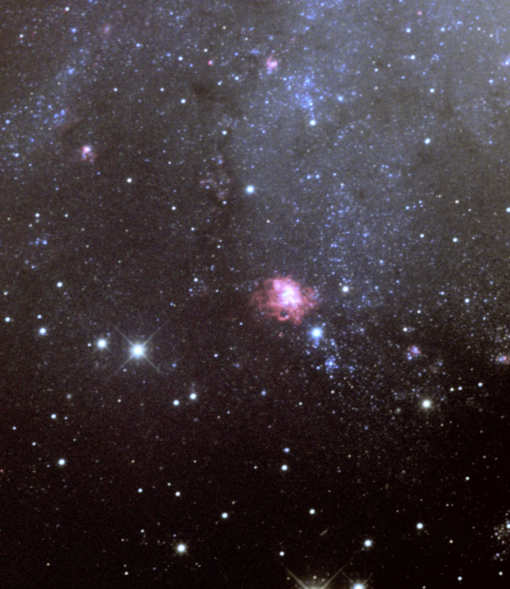
N11, the Bean Nebula
Previously, I imaged the Tarantula Nebula in the Large Magellanic Cloud (LMC). But WISE’s mid-infrared data for this field was saturated/not usable, so I wanted to try another target. I selected the second brightest star-forming region in the LMC, using this amazing photo as a guide. After some digging, I learned that it’s called the Bean Nebula (N11).
I used Stellarium to frame it up, and ended up collecting 24 min of Lum, 48 min of B, 48 min of V, 48 min of R, 196 min of H-alpha, and 144 min of OIII, for a total of 8.5 hours! I also collected a bunch of SII data, hoping to try various tri-color combinations, but alas, its S/N was too low to use.
This was also the first time that I exercised our 32-inch PROMPT-7 telescope at CTIO for astrophotography. I wanted to see how Afterglow Access would hold up against its 4K x 4K detector (fine, just took 4 times longer than normal), and I wanted to see if I could color calibrate its astrophotography Red, Green, and Blue filters as R, V, and B — seems to have worked as well.
I started with a basic LRGB combination (A, below). Then I enhanced the image’s gas content and toned down its (too busy) stellar content. I did this (1) by layering on the H-alpha (Balmer pink) and OIII (blue-green) images, making them as bright as their higher noise levels would reasonably permit (I used the lighten blend mode), and (2) by using the luminance layer to make the stars as dim I could, without losing their colors (B). Lastly, I layered on 12-micron (orange) and 24-micron (blue) mid-IR images from NASA’s WISE spacecraft, using the screen blend mode (C), and cropped/reframed a little to get the final image (D).
The mixture of resolutions, between the optical and IR layers, actually works here, giving the final image a somewhat dreamy feel.


9/11/2022
Messier 83, the Southern Pinwheel Galaxy
Spiral galaxies are blue, and consequently, we should take care to observe them when the moon is down and the sky is dark. However, I wasn’t paying attention, and almost all of the data I got were near full moon :( Let’s process it anyway!
And I’m glad I did, because I’ve been trying to figure out how to correct for the reddening effects of dust in fields like this, and I think I made some progress.
First, I corrected for the relatively minor E(B-V) = 0.039 mag of reddening due to dust in our own galaxy, along the line of sight (A, below). M83’s still too red, but that’s because of dust in M83.
Stars near the surface of M83 won’t be reddened as much as stars deeper in. So how much to correct for? I decided to correct to a depth where half of the B (blue) light is blocked relative to the V (green) light. That’s an additional -2.5log(0.5) = 0.753 mag of E(B-V). The resulting shade of blue looks typical of the O stars that dominate this galaxy’s light (B).
However, this over-corrects stars near the surface of M83, but also over-corrects the bright, typically redder field (foreground Milky Way) stars that are scattered cross the image. Can I have my cake and eat it too?
Yes! (I think.) In both A and B, I corrected the blue and red layers relative to the green layer. But then in C, I take the red layer from A and the blue layer from B. (Technically, I take both red layers and both blue layers, but combine them using the lighten blend mode. But it works out about the same as just taking the red layer from A and the blue layer from B). Color-wise, this looks good!
In D, I layered on my H-alpha data (Balmer pink, highlighting star-heated gas). I had to do it very subtly/carefully, because the data are noisy. But H-alpha data will always be noisy, unless you’re willing to blow through a lot of telescope time (=$). But…
…this field has Spitzer 8-micron data (E). And it’s awesome! At this IR wavelength, you’re looking at star-heated dust, which (on these scales) should be exactly where your star-heated gas is. Plus, it goes much deeper than our (or anyone’s H-alpha data, ever). I added just the tip of this iceberg in F, coloring it the same, Balmer pink color, and it does such a better job.
In the future, I’m going to check Spitzer first before even observing. If there’s good data there, I’m not going to waste the telescope time/$ on H-alpha (when observing galaxies).
So two solid outcomes:
What I’m going to call the “cake” method of RGB combination, for spiral (and irregular?) galaxies, and
With galaxies, Spitzer 8-micron data can be used instead of H-alpha data, to better effect, and at great savings.
Lastly, and just for fun, I blue-green-red combined Spitzer’s 3.6-, 4.5-, and 5.8-micron data. I think these images are pre-calibrated, so I just had to neutralize their backgrounds (G). Stars are still visible at these wavelengths, but since all of these stars’ blackbodies peak at shorter wavelengths, they should all look the same, “thermal” shade of blue that, e.g., O stars look at visible wavelengths. Indeed, this appears to be the case. The redder emission, on the other hand, is from star-heated dust, beginning to crop into the 4.5- and especially 5.8-micron bands.


9/3/2022
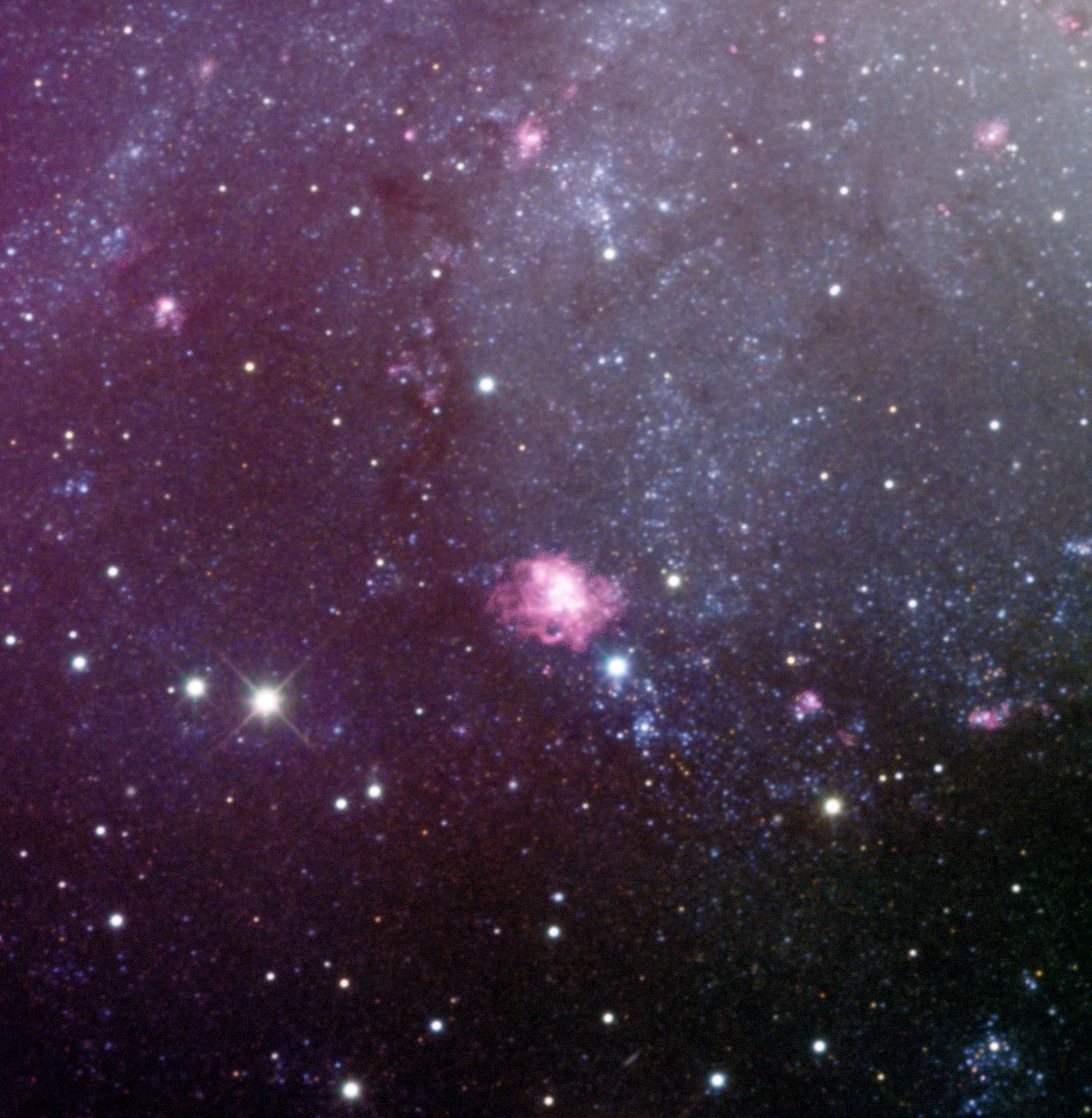
NGC 604, in the Triangulum Galaxy
I know I need to start working on galaxies, but am still kind of hooked on star-forming regions. So I decided to try both — NGC 604 is a massive star-forming region, but not in our galaxy, nor in the Magellanic Clouds, but in the Triangulum Galaxy, the third largest member of the Local Group. So, far away for a star-forming region, but close for a galaxy.
For this observation, I collected about 48 minutes in each of B, V, R, and Lum, and about 96 minutes in H-alpha (also tried OIII, but it didn’t turn out good enough to use).. I collected these observations with Skynet’s 16-inch diameter PROMPT-6 telescope at Cerro Tololo Inter-American Observatory in Chile.
I began by source extracting and catalog calibrating the B, V, and R frames. It turned out very red, because of all of the dust in Triangulum (A, below). I tried many different dust corrections, but I didn’t get the depth of blue that I wanted until I subtracted out a full 2 magnitudes of E(B-V) reddening (B). Note: This does over-correct the foreground stars, and the bright Triangulum stars that aren’t buried as deeply in the dust as the more numerous, fainter stars that I was targeting. I could have just as easily gone with half a magnitude of dust correction, had more colorful foreground stars, but still a lot of reddening across the image.
Then I applied the luminance layer, but couldn’t get a good result until I matched its histogram to the B band’s (C). This makes sense since the faint end of this image is dominated by blue light. Then, I upped the background level a bit, to better bring out the dust lanes.
Then I applied the H-alpha layer, but this one had a poor, noisy background. So I upped its background level a lot, and used the lighten blend mode, which only lets its brighter, better parts through (D). I also tuned down its bright end — I like accentuating these star-forming regions, but there is such a thing as applying too much make up :)
Lastly, I cropped it, to remove the bright star half-on/half-off the bottom of the image (found it distracting).


8/23/2022
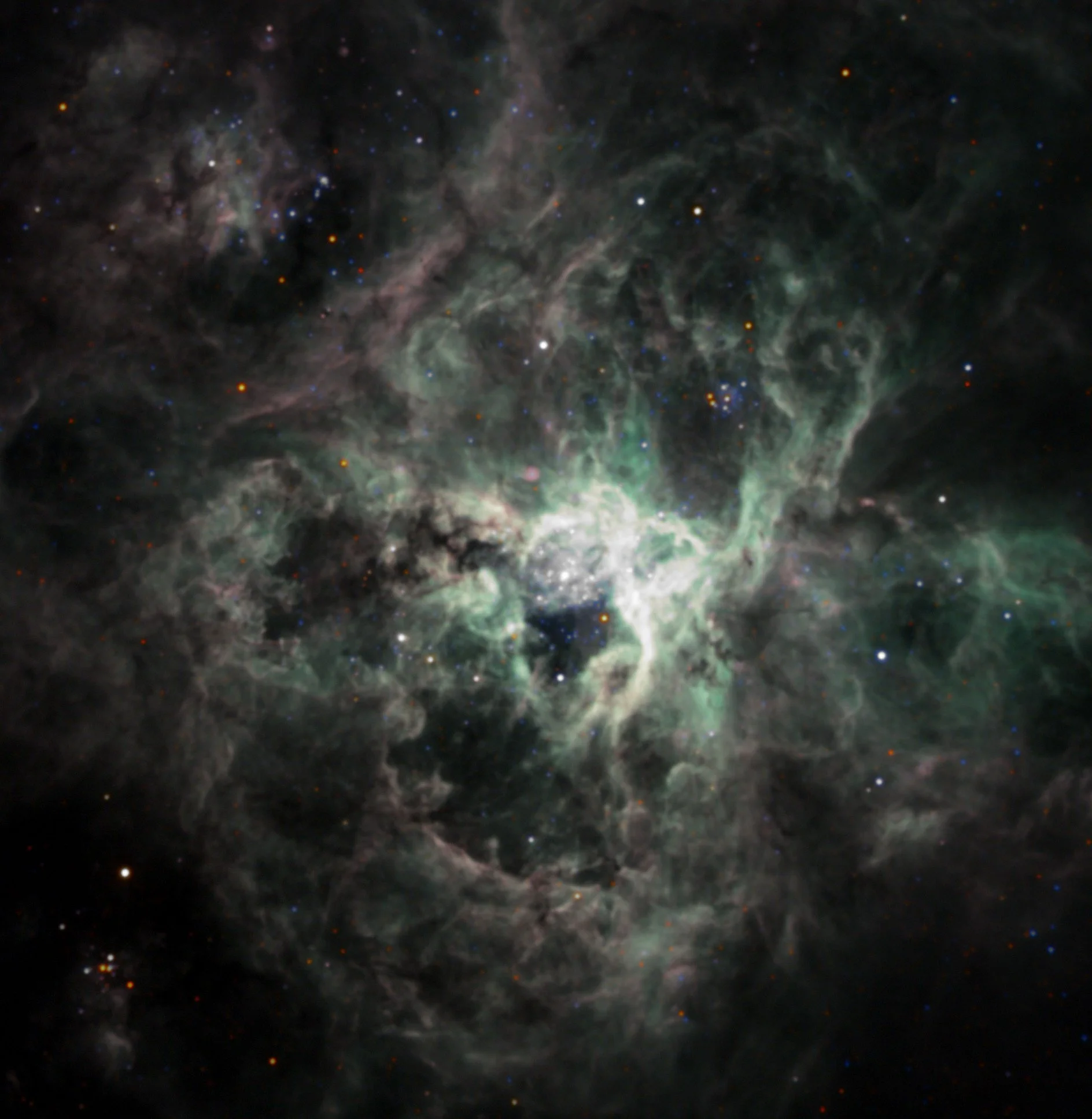
30 Doradus, the Tarantula Nebula
Time to explore narrowband imaging!
I’ve been imaging a number of star-forming regions within the plane of the Galaxy. All are relatively close (else they would be lost behind an accumulation of dust). And if they’re close, you’re exploring a smaller, zoomed-in physical scale. On such scales, you can definitely pick up narrowband emission (such as H-alpha), but not much variation between different types of narrowband emission (e.g., H-alpha vs. OIII vs. SII). For this, you must squeeze a larger physical scale into your telescope’s, fixed, field of view.
In other words, you need to look farther away. And if you don’t want to be swamped by dust, that means you need to look out of the plane. So what’s up there? Other galaxies — but these are too far away to image individual star-forming regions in detail. Globular clusters — but these are old stellar populations, with no gas content / nothing forming now. How about the Magellanic Clouds?
There are lots of star-forming regions in the Magellanic Clouds, and they’re at just the right distance to cram a much larger physical scale into your telescope’s field of view. I decided to start with 30 Doradus — the biggest/most famous of the star-forming regions in the Magellanic Clouds. Using Skynet’s PROMPT-6 telescope, I got 13 min in B, 13 min in V, 13 min in R, 10 min in Clear, 40 min in OIII, and a whopping 161 min in H-alpha. (Sadly, we don’t yet have an SII filter on this telescope — though one’s been ordered!). Now, normally you don’t need this much H-alpha…unless you’re planning something special.
I began with regular catalog calibration of the B, V, and R stacks (A, below). Almost no dust-extinction correction (E(B-V) = 0.066 mag) is required along this line of sight. Then I did something different from what I would do with closer-in star-forming regions. With those, I would first add a luminance layer, to boost the image’s signal-to-noise (S/N) and to adjust its brightness and contrast. Then, I would supplement it / touch it up with an H-alpha layer. But here, narrowband imaging isn’t an afterthought — it’s the objective! So I switch the order:
First, I add the H-alpha and OIII layers, using the “screen” blend mode and our custom “Balmer” and “OIII” colors. Since these cannot be catalog calibrated, I use Afterglow’s next-best option: “neutralize sources”. This adjusts the H-alpha and OIII layers such that the bright end of their histograms match each other, and one of the already calibrated layers. (I reference these to the R layer, because it already includes H-alpha emission, but B or V work about the same.) This boosts the gas content with respect to the stellar content (B vs. A).
Then, I add a luminance layer. In C, I show what a normal, broadband luminance layer does — it emphasizes the stellar content. It’s quite pretty, but also quite busy!
Or…you can do the following: Make a copy of your H-alpha stack and use it again as the luminance layer. This will instead emphasize the gas content with respect to the stellar content. It’s also pretty, but in a starker way. (I’ve always been attracted to desolate, but beautiful places — this has that feel.)
Note 1: This works with regular amounts of H-alpha imaging, but if you zoom in, it will be noisy. This is because H-alpha is a low-S/N filter, vs. Lum or Clear, which are high-S/N filters. If this bothers you, you can compensate by collecting a lot of H-alpha (as I did here!) The extra H-alpha doesn’t really change the underlying color combination, but it does improve the S/N of the final product.
Note 2: I’m still amazed by how good our “Balmer” and “OIII” colors are! Now, if you also had SII, it’s color is pure red — and the combination of red, Balmer, and OIII…probably doesn’t look great. Another option in this case is to color SII red, H-alpha green, and OIII blue — the so-called “Hubble palette”.
Note 3: You could of course skip BVR and just collect narrowband images. In this case, the stars would still be there, but their colors would be wrong. And although they’re not the main point/focus of the image, getting their colors “right” is a nice touch.


8/21/2022
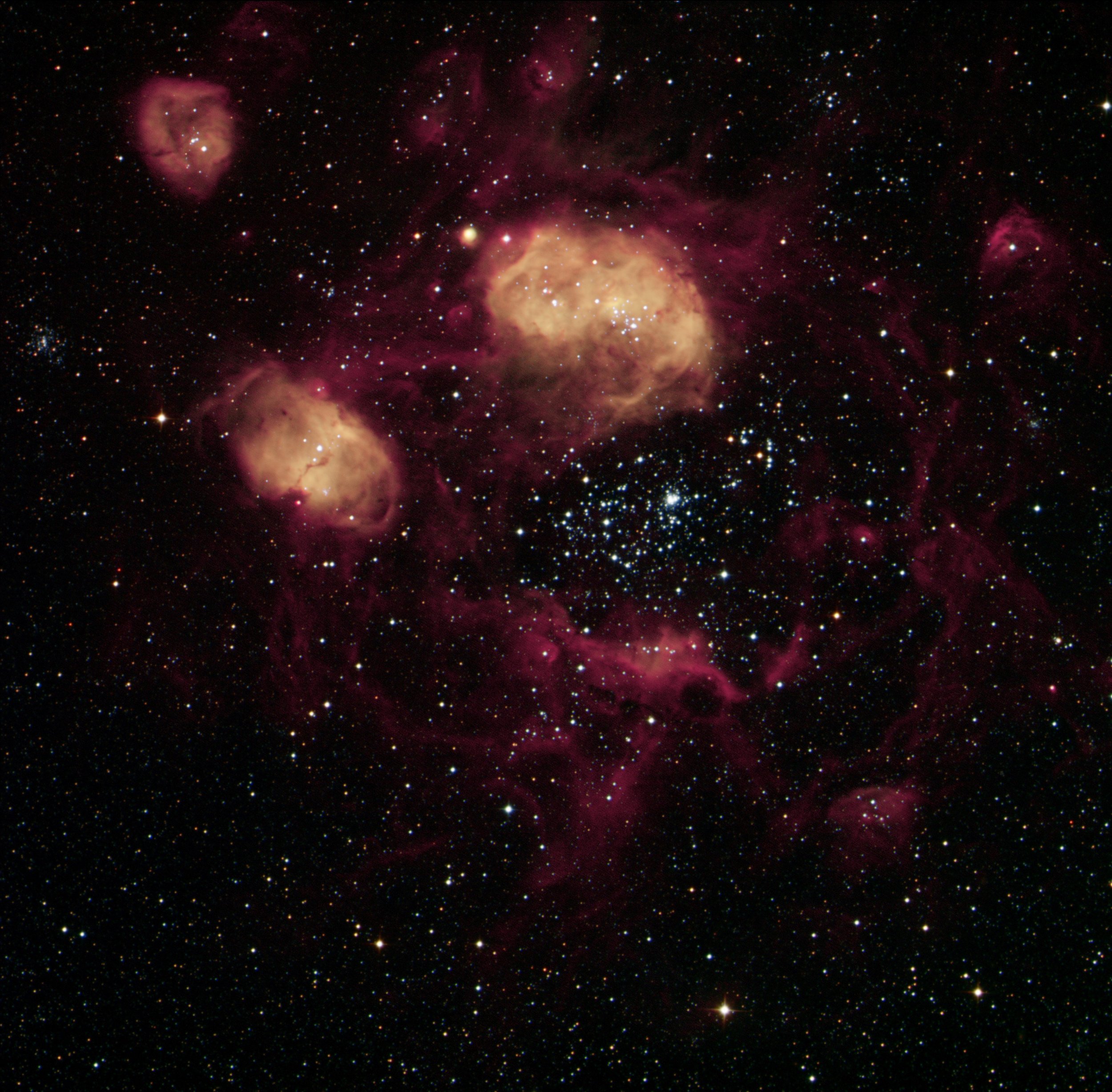
Messier 16, the Eagle Nebula
The point of this blog is how to do student-level astrophotography with Afterglow. This usually means shorter amounts of telescope time, because time on these telescopes is expensive. However, this one is a splurge! I just ran my annual summer program at Green Bank Observatory, and we did a unit on astrophotography. The students were given a couple thousand dollars of telescope time to spend, and they blew about $500 worth on Messier 16, the Eagle Nebula. Together, they collected 63, 54, 54, 36, and 71 minutes in B, V, R, Lum, and H-alpha. So credit in advance to Megan Greensmith, Finn James, Craig Kalkwarf, Nick Konz, Alex Prakken, and Brady Smith!
Learn how to make this image!
Now, they may not have realized it, but this is a very tricky target. There is a lot of dust along this line of sight (E(B-V) = 0.782 mag). Consequently, most images of M16 come out very red. There’s also a lot of H-alpha emission here, which is also red. How to manage it?
First, I made the B, V, R, Lum, and H-alpha stacks. They looked great. Then I began with BVR color combination. I balanced them using source extraction and catalog calibration, with white balance set to “blackbody peaking in B band looks white”. This combo of filters and white balance is about as close to the response of the human eye that we can get with this telescope (Skynet’s 16-inch diameter PROMPT-6 at Cerro Tololo Inter-American Observatory in Chile). And indeed, the combination looks super red (A, below). (I also neutralized the color of the background, which is a default setting.)
But what where the colors of those stars before all that dust reddened them? Professional astrophotographers would try to restore these colors by playing with the white balance. But this is not how the human eye works — our white balance is fixed. Instead, we’ve coded standard dust extinction curves into Afterglow, and the user can remove any amount of dust that they like. Entering E(B-V) = 0.782 mag produced natural looking stellar colors on the first try (B), without having to alter the white balance at all! These are the colors the human eye would see if we were there, instead of looking through all that dust.
Next up is the luminance layer. In B, we’re using a linear stretch mode. The nebulosity is faint, and the stars are blown out. One could use other “simple” stretch modes, like “logarithmic”, “square root”, or “hyperbolic arcsine”, to boost the faint end of the image, but this would blow out the bright end of the image even more. Instead, I used the midtone stretch mode (always use the midtone stretch mode!), which has an extra parameter. Because of this extra parameter (technically called a “control point”), you can boost the faint end and not blow out the bright end (C). Now you can see all of the details in the nebulosity, and the stars look so much better!
After that comes the bonus layers. I began with H-alpha, colored “Balmer pink” — amazing how close we got this color to the real thing! I added it using the “lighten” blend mode, which only adds it to the image if its brighter than what’s underneath. This way you can lay it on without changing the — already natural — colors of the underlying stars. In the end, I added just a bit (D), because I wanted to keep the region around the “pillars” mostly transparent/hazy.
Then I did my “usual” magic trick — I grabbed WISE’s 12-micron band and added it using the “heat” palette” (E). I tried the lighten blend mode, but it reddens it too much, so I used the regular “screen” blend mode. Again, this plays off of the dark, dusty regions perfectly, showing you what parts are being warmed by those bright, blue stars. Note however, parts of this 12-micron field are saturated, and there’s no fixing that — I’ll have to crop the image to exclude these parts in the final step (G).
But first, one more magic trick. I grabbed 2MASS’s 2.15-micron Ks band and added it using the “cool” palette, and the lighten blend mode (F). This shows you where cool, or heavily dust-extinguished, stars are lurking. I don’t like doing this if you can already see the stars in the redder frames, but you can’t in this image. They give the image a feel of confetti, or sprinkles on a cupcake. The whole image feels like a cosmic birthday party :)
Final step — crop to exclude the saturated region in the 12 micron band, and edit out the mild saturation bleeds on the two brightest stars. I did this in MS Paint…because that’s how I roll. OG baby!
Physically, what’s going on here? This region is cool because we have a cluster of relatively new, blue (and other color) stars that formed out of the surrounding gas and dust. They’re heating the gas around them, which is expanding, and pushing up against the surrounding cloud. This lower density, “HII” region is mostly transparent in my image, but closer to the cloud boundaries, you’re also seeing Balmer, and specifically H-alpha, line emission, caused by hydrogen atoms, excited by light from these stars, de-exciting and emitting Balmer photons.
Occasionally, this expanding, heated gas runs up against a slightly denser region, and simply expands around it. This is what causes the “pillars” — the Eagle — as well as the “spire” in the upper left corner. Notice how all of these point back to the hot, blue stars, the source of the expanding shock front. This creates interesting structures, with star-facing sides that are heated and glow at 12 microns, and not-star-facing sides that do not. This is what gives the image its great 3D feel.
Also, once the pillars and spires are carved out, the hot gas starts squeezing them from the sides, eventually causing them to collapse and form more stars. You can see where this might have already happened, in the head of the spire, where a few stars appear to be carving out their own hot gas bubbles.
Lastly, the blue “sprinkles” remind you there’s more to the story, including stars forming inside the cloud, which you cannot normally see. If you look at the bottom center of the image, you’ll see that a few of these stars are heating their surrounding gas and dust, making small “warm dust bubbles” (see the Messier 7 post below). In these cases, both the stars and the bubbles are revealed only through the image’s archival, infrared content.


8/17/2022
Messier 7, the Ptolemy Cluster
I used this target to test color combination in different filter sets. BVR with white balance set to blackbody peaking in B looks natural (A, below). g’r’i’ with white balance set to BB peaking in g’ should look half a spectral class redder (B). Consequently, I tried g’r’i’ with white balance set to BB peaking in V, and indeed, the “natural” color of the bright, blue stars was restored (C). The difference is that dust-reddened stars should be brighter/redder in g’r’i’ than in BVR — and they are (B, C). It’s a nice effect, livening up what were otherwise drab “globular-cluster boring” colors behind the bright blue stars (A).
Learn how to make this image!
This was originally 12 minutes of data from 16-inch diameter PROMPT-5 (1K x 1K). But I saturated the bright stars in every frame (boo!), resulting in vertical bleeding (A, B, C). So I went back for more luminance data, planning to correct the combination in this layer only. I got another 2.1 minutes, this time from 32-inch diameter PROMPT-7 (4K x 4K). I noticed that its diffraction spikes were along the original bleed direction, and 45 degrees rotated from PROMPT-5’s diffraction spikes. So I combined the two luminance layers, (somewhat) hiding the bleeds under the vertical diffraction spikes, and creating this 8-prong diffraction pattern, instead of the typical 4 (D). I like the effect.
Still the image was a little blah. So I added 12-micron (E) and then also a touch of 22-micron (F) IR data from the WISE spacecraft, placing these above the luminance layer, and using the “heat” palette. This shows where stars are warming surrounding dust, and indeed, all of these “warm dust bubbles” landed on the g’r’i’-accentuated, dust-reddened stars (B, C, D) — which makes great physical sense!
I’m really becoming enamored with WISE’s longer-wavelength bands, and its 12-micron band in particular — both for how they can be used to aesthetically improve an image, and for how they can add to an image’s physical story.


