New Statistical Techniques
We have been developing three new, interrelated, statistical techniques. The first has been published as a Ph.D. thesis; we are preparing papers for journal submission, and a web interface, for it now. The second has been published, and we are completing work on a web interface for it now. The third is an offshoot of both, which we will be pursuing next.
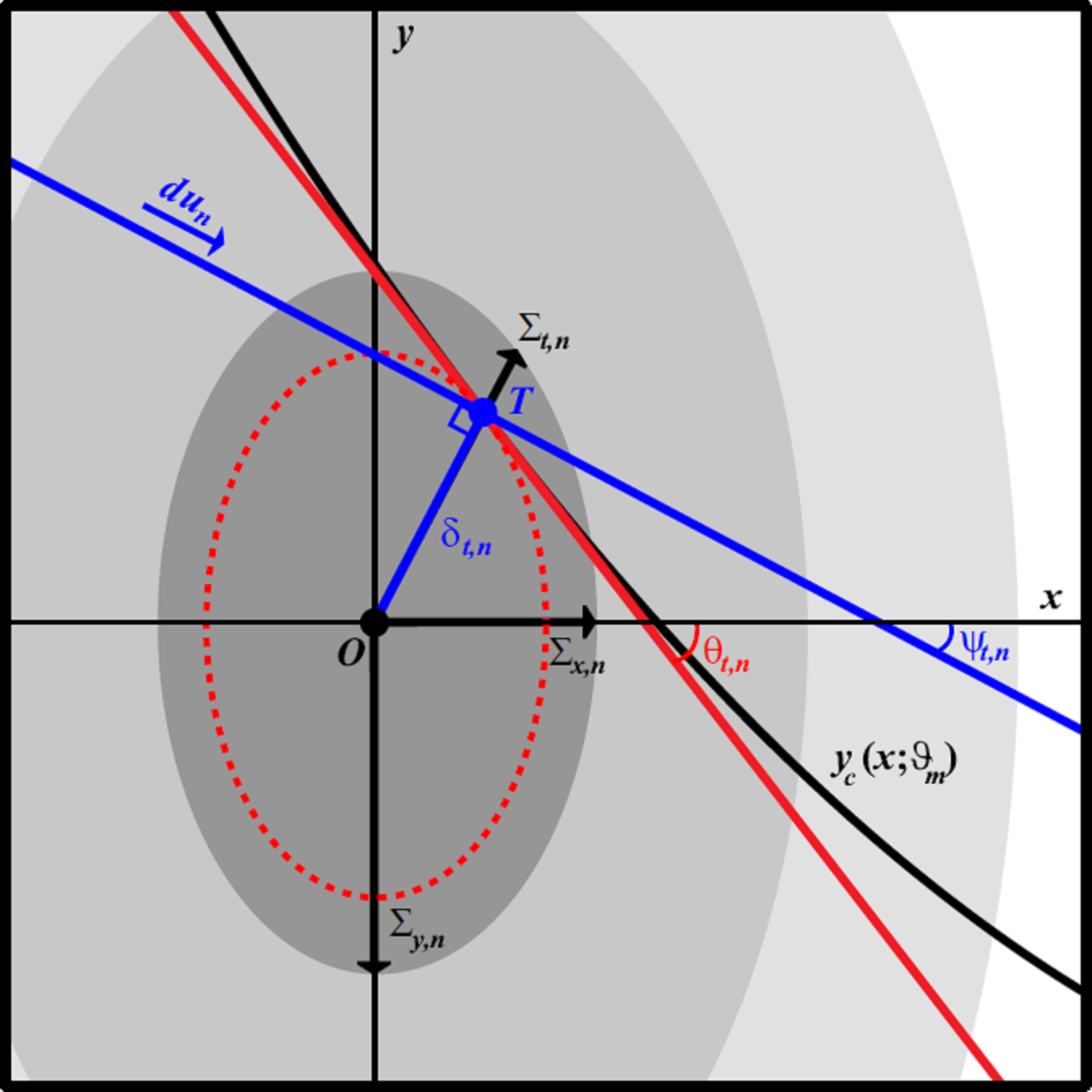
Illustration of the geometry of the TRK statistic. Data point centroid is at (x_n, y_n) (point O), with convolved widths (Sigma_{x,n},Sigma_{y,n}). Model curve y_c(x; theta_m) is tangent to the convolved error ellipse at tangent point (x_{t,n}, y_{t,n}) (point T). Red line is the linear approximation of the model curve, with slope m_{t,n} = tan theta_{t,n}. Blue line indicates the direction du_n of path integration for the TRK statistic, perpendicular to the segment OT. TRK is geometrically equivalent to a 1D chi^2-like statistic measured in the direction of the tangent point.
TRK “Worst-Case” Regression
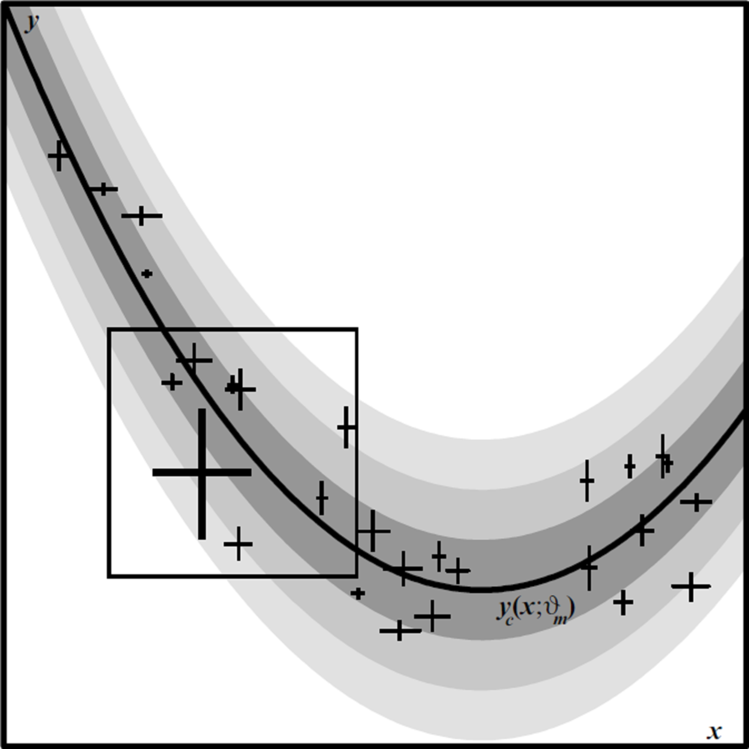
In Trotter’s 2011 Ph.D. thesis, we develop a new, very generally applicable statistic (Trotter, Reichart & Konz, in preparation, hereafter TRK) for fitting model distributions to data in two dimensions, where the data have both intrinsic uncertainties (i.e., error bars) and extrinsic scatter (i.e., sample variance) that is greater than can be attributed to the intrinsic uncertainties alone. A model distribution is described by the convolution of a (possibly asymmetric) 2D probability distribution that characterizes the extrinsic scatter, or “slop”, in the data in both the x and y dimensions with a model curve y_c(x; theta_m), where {theta_m} is a set of M model parameters that describe the shape of the curve. The task in fitting a model distribution to a data set is to find the values of the parameters {theta_m}, and of the parameters that characterize the slop, that maximize the joint probability, or likelihood function, of the model distribution and the data set. First, we derive a very general probabilistic formulation of the joint probability for the case where both the intrinsic uncertainties and the slop are normally distributed. We then demonstrate that there is a choice of rotated coordinate systems over which the joint probability integrals may be evaluated, and that different choices of this rotated coordinate system yield fundamentally different statistics with fundamentally different properties, and yield fundamentally different predictions for any given model parameterization and data set.

Left: Linear fits to a slop-dominated Gaussian random cloud of N = 100 points with zero intrinsic error bars. Point coordinates generated with zero mean, sigma = 1 Gaussian random variables in both dimensions. Solid red line shows fit with D05 statistic; dotted red line is fit with inverted D05* statistic. Blue line shows fit and inverted fit with TRK statistic; for an invertible statistic, the two are the same. Right: Histogram of fitted slope theta for an ensemble of 1000 zero-mean, sigma = 1 Gaussian random clouds of N = 100 points each, for both D05 and TRK statistics. Solid lines indicate expected theoretical distribution. For TRK, p(theta) is a constant; for D05, p(theta) is biased towards theta = 0 by a factor (cos theta)^N.
We show that one choice of rotated coordinates yields the traditional statistic advocated by D’Agostini (2005, hereafter D05), and another the statistic advocated by Reichart (2001, hereafter R01). The D05 statistic is non-invertible, i.e., it yields different model fits depending on whether one chooses to fit a model distribution to y vs. x or to x vs. y. The R01 statistic is invertible, but as we will demonstrate, suffers from a fatal flaw in that it does not reduce to chi^2 in the 1D limiting case of zero extrinsic scatter, and zero intrinsic uncertainty in either the x or y dimensions. We introduce a new statistic, TRK, that is both invertible and reduces to chi^2 in these 1D limiting cases. We demonstrate that the best-fit model distribution predicted by the TRK statistic, in the case of normally distributed intrinsic uncertainties and extrinsic scatter, is geometrically equivalent to the distribution that minimizes the sum of the squares of the radial distances of each data point centroid from the model curve, measured in units of the 1-sigma radius of the 2D convolved intrinsic and extrinsic Gaussian error ellipse.

Left: Linear fits to slop-dominated data. Data points generated by adding independent zero-mean Gaussian random variables with standard deviation sigma_x = sigma_y = 0.5 to N = 100 points randomly distributed between (-1,-1) and (1, 1) along the line y_c(x) = x. Data points are assigned zero intrinsic uncertainties sigma_{x,n) = sigma_{y,n} = 0. Dash-dotted lines: uninverted D05 fit/TRK fit as scale s goes to 0 (shallow line), and inverted D05* fit/TRK fit as scale s goes to 1 (steeper line). Solid blue line: TRK fit at optimum scale. Right: Linear fits to data with both slop and intrinsic uncertainties. The coordinates of each point are the same as on the left. Each point was assigned symmetric intrinsic uncertainties sigma_{x,n) = sigma_{y,n} = 0.25. Dotted red lines: uninverted D05 fit (shallow line), and inverted D05* fit (steeper line); these fits are identical to those on the left. Dashed blue lines: TRK fits at scale s_{min} at which fitted slop sigma_x goes to 0 (shallower line), and at scale s_{max} at which slop sigma_y goes to 0 (steeper line). Solid blue line: TRK fit at optimum scale.
However, unlike the D05 statistic, the TRK statistic is not scalable, i.e., it yields different best-fit model distributions depending on the choice of basis for each coordinate axis. We demonstrate that, in the limit of data that are entirely dominated by extrinsic scatter (i.e., zero intrinsic error bars), the predictions of TRK at extremes of scaling the x and y axes is equivalent to the predictions of D05 under an inversion of the x and y axes. However, D05 is limited to this binary choice of inversion or non-inversion, while TRK is free to explore a continuous range of scales between the two limiting cases. Moreover, when the data are dominated by intrinsic rather than extrinsic uncertainty, the range of scales that result in physically meaningful model distributions is significantly smaller, while the predictions of D05 are the same under inversion whether the data are dominated by intrinsic or extrinsic uncertainty. In the limit of data that are entirely dominated by intrinsic uncertainty (i.e., zero slop), this range of scales reduces to a single physically meaningful scale. We discuss these behaviors in the context of linear model distributions fit to various randomized data sets. We define a new correlation coefficient, R_{TRK}^2, that is analogous to the well-known Pearson correlation coefficient R_{xy}^2, and describe an algorithm for arriving at an “optimum scale” for a fit with TRK to a given data set, which yields linear fits that fall approximately midway between the inverted and non-inverted D05 fits. Lastly, we generalize this algorithm to non-linear fits, and to fits to data with asymmetric intrinsic or extrinsic uncertainties.
Robust Chauvenet Outlier Rejection
Introduction, from Maples et al. (2018)
Consider a sample of outlying and non-outlying measurements, where the non-outlying measurements are drawn from a given statistical distribution, due to a given physical process, and the outlying measurements are sample contaminants, drawn from a different statistical distribution, due to a different, or additional, physical process, or due to non-statistical errors in measurement. Furthermore, the statistical distribution from which the outlying measurements are drawn is often unknown. Whether (1) combining this sample of measurements into a single value, or (2) fitting a parameterized model to these data, outliers can result in incorrect inferences.
There are a great many methods for identifying and either down-weighting (see §2.1) or outright rejecting outliers. The most ubiquitous, particularly in astronomy, is sigma clipping. Here, measurements are identified as outlying and rejected if they are more than a certain number of standard deviations from the mean, assuming that the sample is otherwise distributed normally. Sigma clipping, for example, is a staple of aperture photometry, where it is used to reject signal above the noise (e.g., other sources, Airy rings, diffraction spikes, cosmic rays, and hot pixels), as well as overly negative deviations (e.g., cold pixels), when measuring the background level in a surrounding annulus.
Sigma clipping, however, is crude in a number of ways, the first being where to set the rejection threshold. For example, if working with ≈100 data points, 2-sigma deviations from the mean are expected but 4-sigma deviations are not, so one might choose to set the threshold between 2 and 4. However, if working with ≈10^4 points, 3-sigma deviations are expected but 5-sigma deviations are not, in which case a greater threshold should be applied.
Chauvenet rejection is one of the oldest, and also the most straightforward, improvement to sigma clipping, in that it quantifies this rejection threshold, and does so very simply (Chauvenet 1863). Chauvenet’s criterion for rejecting a measurement is NP(>|z|) < 0.5, (1) where N is the number of measurements in the sample, and P(>|z|) is the cumulative probability of the measurement being more than z standard deviations from the mean, assuming a Gaussian distribution. We apply Chauvenet’s criterion iteratively, rejecting only one measurement at a time for increased stability, but consider the case of (bulk) rejecting all measurements that meet Chauvenet’s criterion each iteration in §5. In either case, after each iteration (1) we lower N by the number of points that we rejected, and (2) we re-estimate the mean and standard deviation, which are used to compute each measurement’s z value, from the remaining, non-rejected measurements.
However, both traditional Chauvenet rejection, as well as its more-general, less-defined version, sigma clipping, suffer from neither the mean nor the standard deviation being “robust” quantities: Both are easily contaminated by the very outliers they are being used to reject. In §2, we consider increasingly robust (but decreasingly precise; see below) replacements for the mean and standard deviation, settling on three measures of central tendency (§2.1) and four measures of sample deviation (§2.2). We calibrate seven pairings of these, using uncontaminated data, in §2.3.

Left: 1000 measurements, with fraction f_1 = 1 - f_2 drawn from a Gaussian distribution of mean mu_1 = 0 and standard deviation sigma_1 = 1, and fraction f_2 = 0.15 (top) and 0.85 (bottom), representing contaminated measurements, drawn from the positive side of a Gaussian distribution of mean mu_2 = 0 and standard deviation simga_2 = 10, and added to uncontaminated measurements, drawn as above. Mode (black line) and 68.3-percentile deviations, measured both below and above the mode, using technique 1 from §2.2 (red lines), using technique 2 from §2.2 (green lines), and using technique 3 from §2.2 (blue lines). The mode performs better than the median or the mean, especially in the limit of large f_2. The 68.3-percentile deviation performs better when paired with the mode, and when measured in the opposite direction as the contaminants. Right: After iterated Chauvenet rejection, using the smaller of the below- and above-measured 68.3-percentile deviations, in this case as measured by technique 1 from §2.2. Techniques 2 and 3 from §2.2 yield similar post-rejection samples and mu and sigma measurements.
In §3, we evaluate these increasingly robust improvements to traditional Chauvenet rejection against different contaminant types: In §3.1, we consider the case of two-sided contaminants, meaning that outliers are as likely to be high as they are to be low; and in §3.2, we consider the (more challenging) case of one-sided contaminants, where all or almost all of the outliers are high (or low; we also consider in-between cases here). In §3.3, we consider the case of rejecting outliers from mildly non-Gaussian distributions.

Flowchart of our algorithm, without bulk pre-rejection (see Figure 30). The most discrepant outlier is rejected each iteration, and one iterates until no outliers remain before moving on to the next step. mu and sigma (or sigma_- and sigma_+, depending on whether the uncontaminated distribution is symmetric or asymmetric, and on the contaminant type; Figure 19) are recalculated after each iteration, and the latter is multiplied by the appropriate correction factor (see Figure 29) before being used to reject the next outlier. mu and sigma (or sigma_- and sigma_+) may be calculated in different ways in different steps, but how they are used to reject outliers depends on whether the uncontaminated distribution is symmetric or asymmetric, and on the contaminant type, and consequently does not change from step to step (Figure 19).
In §3, we show that these increasingly robust improvements to traditional Chauvenet rejection do indeed result in increasingly accurate measurements, and they do so in the face of increasingly high contaminant fractions and contaminant strengths. But at the same time, these measurements are decreasingly precise. However, in §4, we show that one can make measurements that are both very accurate and very precise, by applying these techniques in sequence, with more-robust techniques applied before more-precise techniques.
In §5, we evaluate the effectiveness of bulk rejection, which can be significantly less demanding computationally. In §6, we consider the case of weighted data. In §7, we exercise both of these techniques with an astronomical example.
In §8, we show how RCR can be applied to model fitting, which first requires a generalization of this, traditionally, non-robust process. In §9, we compare RCR to Peirce rejection (Peirce 1852; Gould 1855), which is perhaps the next-most commonly used outlier-rejection technique (Ross 2003). Peirce rejection is a non-iterative alternative to traditional Chauvenet rejection, that can also be applied to model fitting, and that has a reputation of being superior to traditional Chauvenet rejection.
Summary, from Maples et al. (2018)
The most fundamental act in science is measurement. By combining multiple measurements, one can better constrain a quantity’s true value, and its uncertainty. However, measurements, and consequently samples of measurements, can be contaminated. Here, we have introduced, and thoroughly tested, an approach that, while not perfect, is very effective at identifying which measurements in a sample are contaminated, even if they constitute most of the sample, and especially if the contaminants are strong (making contaminated measurements easier to identify).
In particular, we have considered:
Both symmetrically (§3.1) and asymmetrically (§3.2) distributed contamination of both symmetrically (§3.1, §3.2, §3.3.2) and asymmetrically (§3.3.1) distributed uncontaminated measurements, and have developed robust outlier rejection techniques for all combinations of these cases.
The tradeoff between these techniques’ accuracy and precision, and have found that by applying them in sequence, from more robust to more precise, both can be achieved (§4).
The practical cases of bulk rejection (§5), weighted data (§6), and model fitting (§8), and have generalized the RCR algorithm accordingly.
Finally, we have developed a simple web interface so anyone can use the RCR algorithm. Users may upload a data set, and select from the above scenarios. They are returned their data set with outliers flagged, and with mu_1 and sigma_1 robustly measured. Source code is available here as well.

Left: Equally weighted measurements, drawn from a Gaussian distribution of mean y(x) = x and standard deviation 1, where half of the measurements have been contaminated, in the positive direction. Right: Model solutions, calculated from each pair of measurements in the left panel, for the model y(x) = b + m(x - xbar), where xbar = (Sum_i^N w_ix_i) / (Sum_i^N w_i) = (Sum_i^N w_ix_i) / N ≈ 0. Each calculated parameter value is weighted, as prescribed in §2.1, and darker points correspond to model solutions where the combination of these weights, (w_b^{-1} + w_m^{-1})^{-1}, is in the top 50%. The purple circle corresponds to the original, underlying model, and in both panels, red, green, and blue correspond to the weighted mean, median, and mode, respectively, of the calculated parameter values, as defined in §2 and §3. Red also corresponds to least-squares regression, applied to the measurements in the left panel (see §2). The weighted mode performs the best. The weighted mean/least-squares regression performs the worst.
Parameter-Space Regression
In Maples et al. (2018), we introduced a new way of thinking about parametric regression: Given N weighted measurements, and an M parameter model, we calculated separate model solutions for all N!/[(N-M)!M!] combinations of measurements. Each model solution consisted of (1) a value for each of the model’s M parameters, and (2) a weight for each of these values, calculated from standard propagation of uncertainties. We then defined ways of taking (1) the weighted median and (2) the weighted mode of these parameter values, for each parameter, to get best-fit models that are significantly more robust (i.e., less sensitive to outliers) than what one gets by performing least-squares regression on the measurements.
This is a new way of thinking about regression – as something that takes place in a model’s parameter space, instead of in the measurement space. In fact, in Konz et al., in preparation, we show that least-squares regression, performed on measurements, is mathematically equivalent to taking the weighted mean of these parameter values, for each parameter. In this sense, least-squares regression is but one, limited, option, corresponding to the simplest thing one might try in parameter space.
In Maples et al. (2018), we have already presented two, more-robust examples of things one might try in parameter space. But many other possibilities exist. We briefly discuss what some of these possibilities might be, and in particular, how the options presented in Maples et al. (2018) could be improved upon in the future.
We also discuss how parameter uncertainties can be trivially measured in this new formalism, and how prior information can be incorporated just as easily.
Finally, in Maples et al. (2018), we considered only uncertainties in the dependent variable. Here, we show how uncertainties in both dependent and independent variables can be simultaneously, and again, trivially, incorporated in this new formalism. We also address how (1) asymmetric and (2) systematic uncertainties in each of these variables can be incorporated.