
MWU! Blog of Blogs(!)
Astrophotography of the Multi-Wavelength Universe!, or MWU! for short, is a unique curriculum being developed by approximately two dozen institutions, funded by a $3M DoD National Defense Education Program (NDEP) award. MWU! students gain access to optical and radio telescopes around the world, and use them when the pros aren’t to carry out their own investigations of the visible and invisible universe — often creating scientific works of art in the process. They also learn how to effectively communicate their results in the form of a blog, written for other astro-interested students.
MWU! instructors forward their students’ best work for consideration here, in the “MWU! Blog of Blogs(!)”. It’s not just about producing a great image or result, but about producing a great explanation — detailed but concise, using an informal / conversational / approachable writing style.
If interested in offering Skynet’s OPIS! and MWU! curricula at your institution, email introastro@unc.edu.

5/20/2023
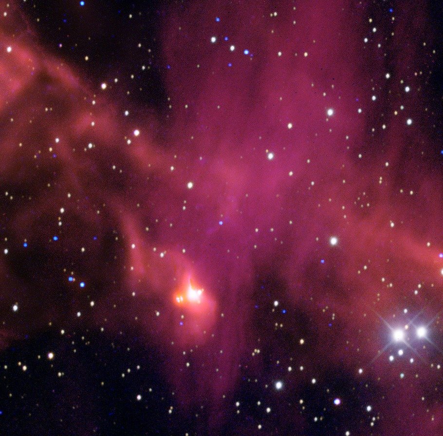
Medusa Nebula
Virgil Walters, Andreas Buzan, Alyssa Manus, and Ruby McGhee
UNIVERSITY OF NORTH CAROLINA AT CHAPEL HILL
About the Image
OVERVIEW
We observed the Medusa nebula which is a planetary nebulae characterized by old red giant stars that eject ionized gas creating the nebula’s luminescent shell. The faint hot blue core is called a white dwarf made of exposed carbon and oxygen which ionizes the surrounding previously ejected gas. Free electrons collide and excite the elements: HI, OIII, and SII and then they de-excite and emit narrowband emission lines. Our images consist of LRGB, narrowband (NB) and incorporated mid-infrared (MIR) archival layers.
For our observations, we used the telescopes PROMPT5 and PROMPT7. For PROMPT 7, we used the filters SII, OIII and Halpha, with an exposure length of 600 seconds per filter. For PROMPT5, we used the filters Lum, B, V, and R, with the following observing times for each filter:
(table)
INFRARED DATA
We first opened all of the files in Afterglow. After checking to make sure our R, V, B, Lum, and narrowband exposures (Halpha, OIII, SII) came out clear, we aligned all of our images using WCS mode. Next, we began making our stacks for the R, V, B, and Lum filters. We used chauvenet rejection with a high and low of 1 and enabled Propagate Mask. Then, we group all of the stacks, as well as the Halpha, OIII, and SII layers, into one image. We then used SkyView Virtual Telescope to gather Wise 12 and Wise 22 data. We colored the Wise 12 data with the “heat” color map and Wise 22 with the cool “color” map. Afterwards, we used IRSA (Infrared Science Archive) to gather Spitzer data. We collected observations from the IRAC 4 telescope, which gathers wavelengths at the 8 micron level, which is similar to the Wise 12 data collecting hot gas information, and colored it with the “balmer” map. We aligned and cropped these images the exact same way as with the optical filters except for changing the blend mode to lighten so they add to the already-existing optical layers instead of partially replacing them.
For more info: https://tarheels.live/astr110wwalters/medusa-nebula/

5/10/2023
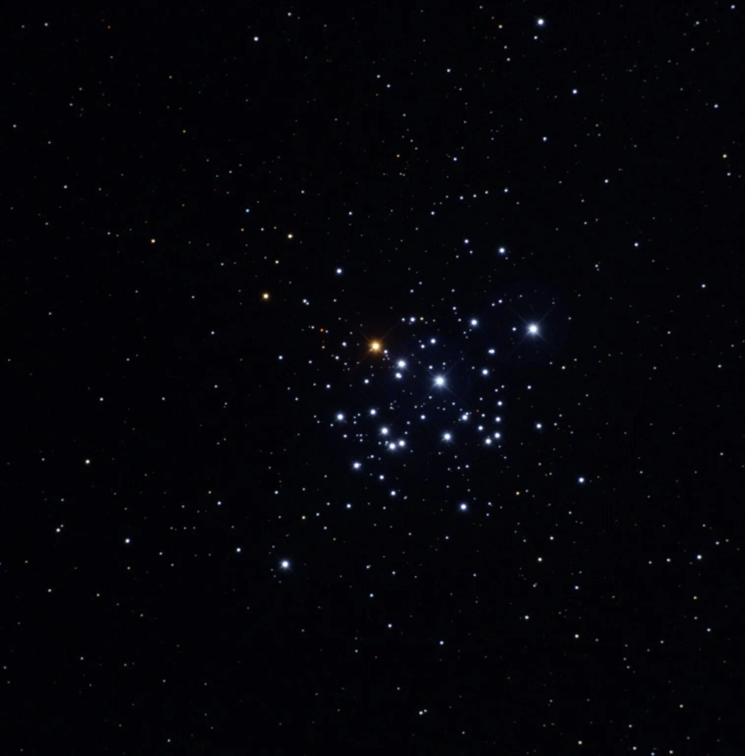
About the Rosette Nebula
Adrienne Brummett, Carlee Markle, and Christina Hollyday
UNIVERSITY OF NORTH CAROLINA AT CHAPEL HILL
For this module, our group chose to image NGC 2244, aka the Rosette Nebula. The Rosette is a star-forming HII region located in our own Milky Way Galaxy. It is within the Monoceros region of our galaxy and contains enough gas and dust to produce 10,000 stars like our Sun. It has a circular shape and a deep dark center, causing it to be named after a flower. This shape is caused by its core containing massive stars whose radiation and flows of charged gas particles have blasted a hole through the material.
Observations
We had to place multiple rounds of observations to fully compile enough data to do the Rosette Nebula some justice. The Rosette Nebula is too large/close to be fully observed by our telescopes so we had to go into Stellarium and look up our target and just choose one specific DEC/RA region to image.
Our first observation was placed by Christinia Hollyday on PROMPT-6 who captured the following RVB+Lum test observation data:
For more info: https://tarheels.live/abrumastro/2023/04/17/about-the-rosette-nebula/
5/7/2023
The Birth of Stars: Using Multi-Wavelength Photography to Understand Star-Forming Regions
Nat Heddaeus, James Thompson, and Rujula Yete
UNIVERSITY OF NORTH CAROLINA AT CHAPEL HILL
Observation Details
We observed the star-forming region (SFR) IC 2944, also known as the Running Chicken Nebula. Observations were made using the PROMPT-5 Telescope, stationed at Cerro Tololo Inter-American Observatory, Chile. We used the visible light filters R,V,B and Lum (Red, Green, Blue, and Luminance; observation credit to Rujula Yete), with observing times of 100, 150, 200, and 90 seconds respectively, and the narrowband filters Halpha and OIII (observation credit to James Thompson), with 600 second observing times for both filters.
Image Processing
Once our images came back, per usual they were cleaned, aligned, and stacked by their respective filters. For our star forming region, we used R,B,V, and Luminance filters, Halpha and OIII narrowband filters, and some supplemental infrared filters which we will discuss later.
For more info: https://tarheels.live/astrorujula/2023/04/20/the-birth-of-stars/

5/3/2023
Star Clusters & Ages
Kayley Hawryliw
University of Saskatchewan
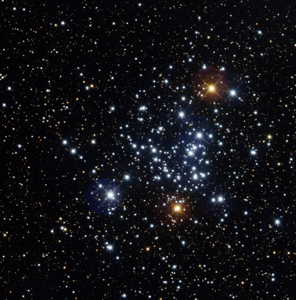
NGC 4755, also known as “The Jewel Box” cluster, is a young, open star cluster in the Constellation Crux located in the southern sky. NGC 4755 is approximately 6,440 lightyears from earth, with a Right Ascension of 12h53m39.499s and Declination of -60d22m15.6s. Its estimated age is approximately 14 million years and was originally discovered by Nicholas Louis De Lacaille in 1752. It later received the title of “The Jewel Box” cluster in 1854 when observed by John Herschel as he compared the cluster’s appearance to be that of a “superb piece of fancy jewellery.”
The cluster stars make up the shape of a letter ‘A’ that points to the west, with a bright red Supergiant star in the centre. The Milky Way Star Clusters Catalog (MWSC) records the 8 brightest members of the star cluster are B giants and Supergiants, with 23 central stars and 110 cluster stars in total. Unfortunately, as noted on in-the-sky.org, this cluster is not observable from Saskatoon because the cluster is so far in the southern sky and never rises above the horizon, however in the south it appears as a hazy/fuzzy star to the unaided eye.
For more info: https://sites.usask.ca/astro/2023/03/31/ngc-4755-the-jewel-box-cluster/

4/27/2023
Star Clusters & Ages
Saki Male, Nathan Flinchum, Delanie Mitchell, and Mia Mese
University of North Carolina at Chapel Hill
Stars are some of the brightest, most beautiful, and complex entities that encompass our vast cosmos. The life cycle of a star is that of an intricate, transformational, and extensive process. The various processes of changes that a star goes through in its magnanimous life is known as stellar evolution. In this module, we will look at three distinct star clusters and process, analyze, and compare them to uncover key properties about the clusters such as age, color, luminosity, and temperature.
For more info: https://tarheels.live/delaniesouterspace/2023/03/23/star-clusters-ages/

4/25/2023
Pulsars and Polarization
Delanie Mitchell, Saki Male, Nathan Flinchum, and Mia Mese
University of North Carolina at Chapel Hill
Neutron stars… Pulsars… What’s it to you? Well, if you’re anything like us, you’re pretty interested in detecting them and their polarization. But wait, what is all of this? Well, first off, a neutron star is a remnant of a supergiant star and is very dense. This is normally the stage that follows the collapse of a supergiant as it has run out of fuel—causing its core to collapse and become a neutron star. Then, pulsars are basically neutron stars that continuously rotate (sometimes at very rapid speeds) and emit radiation in intervals. Also, as neutron stars are relatively, pretty small (some the size of U.S. states) we are unable to detect at optical wavelengths due to the thermal source being proportional to the size of the star. This is why we are dove into utilizing the pulsar’s magnetic fields to detect them, along with their periods. So, in summary, we are talking about a neutron star’s magnetic fields, measuring their pulse periods, and seeing if the detected pulse is polarized or not!
For more info: https://tarheels.live/miasmerrymultiverse/2023/04/05/pulsars-and-polarization/

4/21/2023
Pulsars in the Radio
Virgil Walters, Andreas Buzan, Alyssa Manus, and Ruby McGhee
University of North Carolina at Chapel Hill
Data Collection
We used Skynet’s 20m-diameter radio telescope at Green Bank Observatory to detect the pulsars PSR 1919+21 and PSR 0950+08 and used the substitute data provided by Skynet user bddean21 for PSR 0329+54, since our initial observation was unsuccessful and did not load into the graph. We can do this even if pulses are below the noise level by measuring the pulsar’s rotation-period and then producing period folded pulse profiles. Then we tried to detect if the signal is polarized for the brightest pulsar, PSR 0329+54: this would rule out thermal emission which is never polarized, but non-thermal emission involving magnetic fields can be highly polarized. Lastly using the period measurements, we placed an upper limit on the size of pulsars or neutron stars.
For more info: https://tarheels.live/astr110wwalters/pulsars/

4/18/2023
Module 1C: Optical Planetary Imaging
Karsen Kitchen
University of North Carolina at Chapel Hill
In this module, we captured the planets within our solar system with optical planetary imaging. The goal of this module was to try to capture the authentic color of the planet, as if we were seeing it from space ourselves. We don’t have enough time or resources to make a high-definition, professional optical telescopic picture of our planets, but we’ve got Skynet and a dream! Through using Skynet and Afterglow, we managed to capture images of Jupiter, Neptune, Uranus, and Mars. At the time we put the photographs in, Saturn and a couple of other planets were too close to the sun to be properly photographed, but thankfully, Dr.Reichart had put in some premature observations for us.
Using Skynet, we set our target and used the same settings we used to photograph the moon: Max sun elevation to -12, min target elevation to 30, and max moon phase to 100. In hopes that one of the planets near the sun makes a short appearance, we set out min visible hours to 0.25, and put min moon separation to 30.
For more info: https://tarheels.live/karsenkitchen/2023/02/15/module-1c-optical-planetary-imaging/
4/16/2023
Stellar Evolution
Nat Heddaeus, James Thompson, and Rujula Yete
University of North Carolina at Chapel Hill
To explore the process of stellar evolution, our group observed three star clusters of different ages. NGC 3293 (observation credit to Nat Heddaeus) was classified as a young cluster. NGC 5316 (observation credit to Rujula Yete) was classified as an intermediate aged, or open cluster. NGC 4833 (observation credit to James Thompson) was classified as a globular, or old cluster. Comparison of these three clusters demonstrates the relationship between a stellar cluster’s age and colors.
Observation
Our young cluster, NGC 3293, was observed via the PROMPT-6 remote telescope. Our intermediate and globular clusters, NGC 5316 and NGC 4833 also used PROMPT-5 in addition to PROMPT-6. Both telescopes reside at the Cerro Tololo Inter-American Observatory, Chile. All three clusters were imaged on January 27, 2023. As we observed the clusters in late January, observations were limited to a right-ascension (RA) of ~3-13. The clusters were observed RA’s of:
NGC 3293: 10:35:49.20
For more info: https://tarheels.live/nhastrophotography/2023/03/25/stellar-evolution/

4/10/2023
Lunar Light
Nathan Flinchum
University of North Carolina at Chapel Hill
Radio: It’s more than AM/FM songs to listen to while you drive! It’s light! As a reminder, radio is a long-wavelength section of the electromagnetic spectrum. Although these observations were not taken in optical wavelengths, I was still able to make use of the radio data (with Skynet’s radio cartographer algorithm) to create a few radio images with (arbitrary) colors!
For more info: https://tarheels.live/nflinchum/2023/02/06/lunar-light/

4/7/2023
The Moon’s Light
Rianne Eccleston
University of North Carolina at Chapel Hill
The brightness of the moon, as seen from Earth, varies drastically throughout its different phases. The light we see is reflected from the sun as it lights up different portions of the moon. However, there is a common misconception that the moon does not emit any light itself. There is a thermal emission coming from deep within the lunar soil, which we cannot see. This is because the moon is emitting light within the radio wavelength, invisible to the human eye. This can be proved using a radio telescope and measuring the radio brightness of the moon over a period of time.
To collect our data, we used the 20-meter radio telescope at Greenbank Observatory in West Virginia. Radio telescopes are giant pieces of machinery, but this one is considered small, only four times larger than the world’s largest optical telescope. That being said, they are also quite complex and delicate; things don’t always work to plan. I submitted an observation of the moon but it never came back, so I had to analyze my groupmate’s data.
For more info: https://tarheels.live/throughthetelescope/2023/02/07/the-moons-light/

4/5/2023
Star Clusters
Alyssa Manus
University of North Carolina at Chapel Hill
For this project, my group and I entered observations for three star clusters of different ages, created H-R diagrams to estimate age, metallicity, and other factors, as well as making comparing the H-R Diagrams to our images and seeing how well they align.
Observations
For NGC 3293, the young cluster, we used the telescope PROMPT 6. We took a total of 5 exposures per filter with 30-minutes delays between each set of B, V, R, and I filters. The total observing time for each filter are as follows: B = 31.5 seconds, V = 23.6 seconds, R = 11.8 seconds, and I = 23.6 seconds. The reasoning for spreading out our exposure times is to a) prevent “ghost” images of brighter objects that may be captured in the observation and b) allow other classmates time to collect their data as well!
For NGC 3330, the intermediate cluster, we used the telescope PROMPT 6. We took a total of 5 exposures per filter with 30-minutes delays between each set of B, V, R, and I filters. The total observing time for each filter are as follows: B = 118.1 seconds, V = 59.05 seconds, R = 78.75 seconds, and I = 59.05 seconds. The exposure lengths for each filter vary because we need to collect quality data that consists of just enough time to capture the cluster’s dimmer stars without overexposing the brighter stars. This allows us to collect the unique photometric measurements through the wide array of magnitudes that each cluster contains.
For more info: https://alyssacmanus.wixsite.com/astrophotography/post/star-clusters
4/3/2023
Stellar Evolution
Unique Davis, Ryan Brown, Henry Nachman, and Georgia Phillips
University of North Carolina at Chapel Hill
Star Clusters
The universe is filled of stars with intricate properties and unique origins. Stars that exist in a cluster will have similar ages so by imaging the cluster, we can observe its properties and determine an age for the cluster. In this blog post, our group will analyze and identify properties of three star clusters in our cosmos: IC 2948 (young), NGC 3766 (intermediate), and NGC 3960 (old).
To observe NGC 3960, we used Skynet’s Prompt 6 telescope with the following filters and exposure times:
(table)
To observe NGC 3766 we used Skynet’s Prompt 6 telescope with the following filters and exposure times:
(table)
To observe IC 2948 we used Skynet’s Prompt 6 telescope with the following filters and exposure times:
For more info: https://tarheels.live/gphillipsastrophotography/2023/03/29/stellar-evolution/

3/29/2023
The Moon in Radio
ClairE Helms
University of North Carolina at Chapel Hill
Taking optical images of the night’s sky is one task; capturing celestial objects in other wavelengths is another beast. You may not realize imaging sky in radio is even possible – but not only is it possible, it’s very useful! “Seeing” the sky in radio allows astronomers to discover objects not visible to the human eye or optical telescopes. Some distant objects, for example, are impossible or difficult to see in the visible light spectrum because of visual obstructions like dust and gas clouds. Radio waves, however, can penetrate these obstacles because they have a longer wavelength than visual light! Radio observing is also very practical because it can be done in daylight and through clouds, unlike optical observing. Other benefits we will explore later include radio astronomy’s ability to detect polarization and emittance variance of objects in real time.
For more info: https://clairehhelms.github.io/posts/moon-radio/

3/27/2023
Taking the Moon’s Temperature
James Thompson
University of North Carolina at Chapel Hill
When we talk about “light”, we’re usually referring to the visible light we see with our eyes. However, other, invisible forms of light can also give us equally valuable information about astronomical objects. In our case, we’ll see what we can glean from looking at a familiar object, the moon, via a less familiar form of light: radio waves.
We know that the amount of visible light from the moon varies significantly over time, as the moon changes its phases, so a natural first question to ask is whether the brightness of the moon in the radio spectrum will change in the same way.
To see if this is true, we take two radio images of the moon a few days apart using the 20-meter diameter telescope at the Greenbank Observatory in West Virginia. You might be surprised that we need to so large a telescope to get such coarse-grained observations of the moon.
To understand why such a large telescope is required, we have to consider what determines the resolution of the image we end up with. In general, this is given by θ = 1.22λ/D radians, where λ is the wavelength of the light we’re observing and D is the diameter of our telescope making the observation. Since we’re working in the radio part of the spectrum, our wavelength is very large, about 20 cm, so to get a reasonably small value of θ, D must be large to compensate.
For more info: https://tarheels.live/jamestastrophotography/2023/02/11/41/

3/24/2023
Our Home (Solar) System
Nathan Flinchum
University of North Carolina at Chapel Hill
The Solar System! We know it, we love it, we live in it! Most of us are well aware of what the eight planets of our neighborhood that revolves the sun look like. In this experiment, we take a look at observing (those that are observable) these very planets with an emphasis on colors. The diversity in size, color, and detail is what makes each of them unique. Studying these aspects has been a blast!
1 – Observations
Working together with a group to observe the planets, we split up the tasks. I chose Uranus, Delanie Mitchell was tasked with Mars, and Mia Mese with Neptune. Our group unfortunately did not receive any images back for Jupiter, since the observation window was getting smaller quickly, as the gas giant got closer to being washed out by the sun each day. Therefore, we used our instructor’s (Dan Reichart) images of Jupiter that he was able to get in time. The other planets weren’t observable unfortunately, as they were also too close to the sun.
For more info: https://tarheels.live/nflinchum/2023/02/17/our-home-solar-system/

3/20/2023
Lunar Imaging: Radio
Mia Mese
University of North Carolina at Chapel Hill
When you think about astrophotography or even astronomy as a whole, most people probably think about optical images. This makes sense as there are things such as planets, nebulae, star clusters, etc. that are beautiful to look at. However, there’s a whole world to be seen outside of these traditional images: the radio world. Observing the universe in the radio wavelength is another interesting way to observe and collect data, and that’s exactly what was done in this module with the Moon. So, let’s find out how to see the Moon in radio and measure its temperature!
Skynet Observations
To start I opened up Skynet and went to radio observing. I searched for the Moon and then made sure to set my Min. Sun Elevation to 10 and my Min. Target Elevation to 20 degrees. One important distinction between me and my groupmates was that I set my observation to be on a 4-day delay, meaning it was dispatched on January 17th as opposed to January 13th when the original moon observations were put in. Next, I moved on to the receiver page. We took this observation using the Greenbank Observatory’s’ 20m’s L-band receiver which has a set range of frequencies ranging from 1300 MHz to 1800 MHz. However, in order to remove frequencies that contain human-made interferences, its necessary to use the HI bandpass filter that restricts the range to 1355 – 1435 MHz. Then it was on to the path page. To create a rectangular radio map, I selected the “map” path type and make sure the map was 6 beamwidths across in both directions. Then I ensured that data was collected every gap of 1/5 beamwidths with an integration time of .3 seconds. Once I double checked to make sure everything was entered correctly, I submitted the observation.For this part of Module 1 we wanted to measure the temperature of the moon and we did this by taking radio observations of the moon and Virgo A and then taking those same observations 4 days later to see the change in temperature. For this I observed the moon 4 days later and this is one of the images that I received back from my radio telescope. We observed the moon between frequencies 1355 and 1435 MHz. Later on, we used Afterglow to measure the flux of each of our images. With this we were able to use Virgo A as a calibration source to measure the flux density of the moon. We found that as the moon’s phase got dimmer the flux density of the moon actually increased which was strange because on an optical telescope or in the sky the moon would be less bright. So, we found the ratio between Virgo A’s flux and the moon’s flux to find out the relative density. We then multiplied that ratio by Virgo A’s flux which we got from Skynet which was a value of 229.2. We used this multiplied by the ratio to get the flux density of the moon. Lastly to find temperature we needed to figure out the distance to the moon from earth for each time of day that we found. With this we could compare the temperature of the moon at 61% full and 20% full. For 61% we got 241 K and for 20% we got 231 K. Even though the temperature of the moon did decrease it wasn’t very significant and for the data we got from the entire class the average temperature was basically identical. This shows that the temperature of the moon that we see in this radio image comes from thermal emission and not from reflected sunlight. We know this because of the lack of temperature change as the amount of sunlight we see reflecting off the moon decreases.
For more info: https://tarheels.live/miasmerrymultiverse/2023/02/08/lunar-imaging-radio/

3/14/2023
Earth’s Moon
Alyssa Manus
University of North Carolina at Chapel Hill
On January 10, 2023, I requested a set of lunar images from Skynet’s PROMPT-MO telescope. The goal was to collect a set of seventy-five total images and “collage” them together to get a full color image of Earth’s moon. This post will walk you through the entire process of collecting, processing, and editing to acquire the final result (shown below).
Observe
The first step was to enter the observation into Skynet’s system of robotic telescopes. Unfortunately, the images that were returned from PROMT-MO had some issues. I used a classmates observation from was PROMPT-5, a telescope from the Cerro-Tololo Observatory in Chile. Thank you Ryan Brown! This telescope has a field of view of ten arcminutes, so he requested a set of 5×5 tiles to align and stack together to create a full mosaic of the moon. He requested a total of 75 images, 25 with each of the three different filters; U, OIII, and Halpha. This allowed me to create a color image.
Process
I uploaded all 75 images into Afterglow to start processing and creating the final image. The first step in Afterglow was to align all 75 images using the Aligner tool. I selected all of the images, enabled Mosaic Mode, Features Mode, and adjusted the Ratio Threshold to 0.3. After that processed, I began the stacking job. Using the stacking tool, I selected the aligned images with the U filter and turned on Multiplicative, Additive, and Global Equalization, and submit the job. I then did the same with the OIII and Halpha filters. Once that was done, I changed the color map from gray to the respective filter colors (Halpha as red, OIII as green, U as blue) and used the midtone stretch mode, which resulted in the three following images.
For more info: https://alyssacmanus.wixsite.com/astrophotography/post/earth-s-moon

3/9/2023
Green Comet (C/2022 E3 ZTF)
Alyssa Manus
University of North Carolina at Chapel Hill
Discovered by the Zwicky Transient Facility in 2022, C/2022 E3 was found to have an orbital period of 50,033 years. This means this green comet only comes around Earth about every 50,000 years. It reached closest to Earth on February 1, 2023 with a distance of 0.28 AU (a little over 1/4 the distance from Earth to the Sun). At this point, it was measured to have an apparent magnitude of about 5. For comparison, the Moon has an apparent magnitude of -12.74, whereas Uranus has a brightness of 5.68, much closer to C/2022 E3. This once in a lifetime (over 500 lifetimes, actually) event happened to take place during a time where we have the technology to image it.
Observing and Processing
I was lucky enough to have a classmate and group member who was able to put in an observation through Skynet's system of robotic telescopes for this spectacular green comet on February 1. Andreas Buzan used Mars Desert Research Station's MDRS-14 telescope to take 10 20 second exposures with the B filter, 10 15 second exposures with the V filter, and 10 10 second exposures with the R filter. Since telescopes take images in black and white, these filters allow us to make a full colored image.
For more info: https://alyssacmanus.wixsite.com/astrophotography/post/green-comet-c-2022-e3-ztf

3/3/2023
Moon
Nat Heddaeus
University of North Carolina at Chapel Hill
Photo-Taking/Making Process
This photo of the moon as seen from the Northern Hemisphere (but taken in the Southern Hemisphere!) was observed on January 11, 2023 using the PROMPT-6. The remote telescope took 27 images, 9 for each filter, with a 3×3 tiling pattern. Each image taken by the PROMPT-6 had a 0.2 second exposure time. The Halpha filter (see image A) observed the moon through the red part of the spectrum. The OIII filter (see image B) observed in the green/blue part of the spectrum, and the U filter (see image C) in the ultraviolet. The images for each filter have been color mapped. The three color mapped images were stacked to create a composite image of the moon (see image D).
Regions of Interest
Using photo editing and Adobe Lightroom, I was able to bring out some of the colors of the moon. The colors tell us about the moon’s minerology.
A. The crater on the leftmost side of the highlighted region is the region known as Aristarchus. Bright blues and dark yellows can be seen surrounding the crater. The yellows (also known as Wood’s Spot), are glass deposits, formed when rock heated by the impact of a meteoroid with the moons surface were cooled by the impact’s ejecta. The blues are also glass deposits, the blue caused by the deposits being rich in titanium. The white spots surrounding Aristarchus are Copernicus and Kepler. They were formed by ejecta from the meteoroid impacts settling over areas with lava flow.
For more info: https://tarheels.live/nhastrophotography/2023/01/27/moon-1-11-23/

2/28/2023
The Light Side of the Moon
Rianne Eccleston
University of North Carolina at Chapel Hill
“One small step for man, one giant leap for mankind.”
These words marked a scientific turning point in human history, when we first stepped foot on a celestial body other than our own. Because of the moon’s close proximity to Earth, it is one of the most studied objects in space. Yet still, it is commonly regarded as a rock of every shade between black and white. The reality is, the moon had a dynamic past, creating a whole range of colors that tell us it’s story. Here’s what we can learn from the moon’s mineralogy.
For more: https://tarheels.live/throughthetelescope/2023/02/02/the-light-side-of-the-moon/
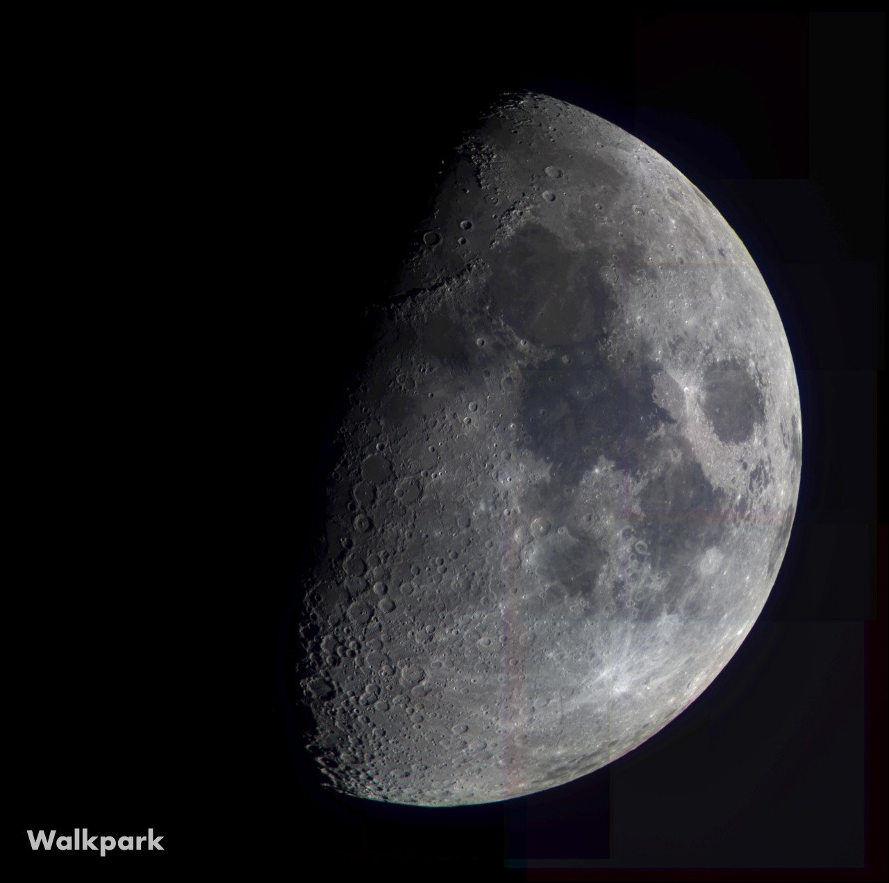
2/24/2023
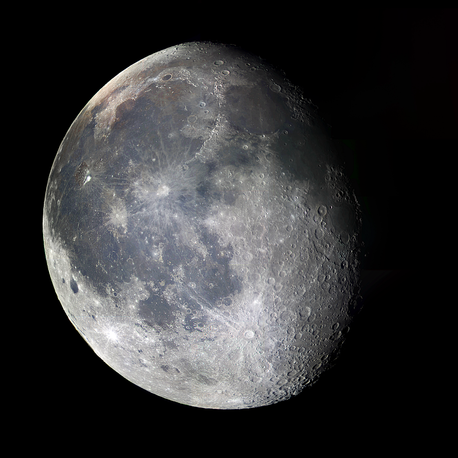
The Moon
Vergil Walters
University of North Carolina at Chapel Hill
About the Image
Overview
This image is a stack of 27 individual images computationally tiled and aligned in the software Afterglow. Three sets of nine images were taken by the optical telescope PROMPT6 in the red, green, and blue spectra; these sets were then combined to form a complete color image like the one above. The final composite image was taken from Afterglow to the photo editing software Photopea for digital enhancement. The primary goal of all edits made was to unobtrusively improve brightness and contrast as well as saturate important areas of color and remove artifacts of the aligning and stacking processes.
PROMPTING PROMPT6
Because the moon is really big in the telescope’s field of view, it was necessary to image the moon in sections the could be aligned later: a three-by-three grid of nine images each was sufficient to capture the whole moon, and with three color filters, there would 27 exposure in total. To ensure the image would not be overexposed due to additional light from the sun, the telescope was instructed to only begin taking exposures when the moon was at least thirty degrees above the horizon, would remain so for half of an hour, and the sun was at least twelve degrees below the horizon. Despite these precautions, initial images returned some improperly exposed areas which will be discussed later.

2/22/2023
Beyond the Aether: The Moon
Jacob BlizzarD
University of North Carolina at Chapel Hill
We all know the moon, Earth’s natural satellite, but it’s hard to see from the ground when looking with the naked eye. Sure, you’re able to catch certain details such as one or many of the Moon’s “seas”, but overall it’s a monotone semi-circle high in the sky.
But with the power of telescopes and Skynet, not the terminator one, we can gain a much better look at our Moon and it’s details. These pictures were taken from several locations on the globe, the telescope I used for my pictures was PROMPT-6, located out in Chile. But the telescope I had originally intended to use was NSO, which is in Vermont, is not run by Skynet, and was down for maintenance when I needed the pictures.
For more: https://tarheels.live/jblizzastr110/beyond-the-aether-the-moon/

2/20/2023
The Moon in Color
James thompson
University of North Carolina at Chapel Hill
Though the moon may seem like a dull and barren world, especially when compared to the Earth, it actually had a tumultuous history. By looking closely at photographs of the moon taken by powerful Earth-based telescopes, we can bring some of this history to life. Ultimately, we’ll end up with the image below, and you’ll have learned how it was made and what subtle info about the moon’s past it hides:
To start, we need to photograph the moon. The telescope we’re using, called the Prompt-5, is located at the Cerro Tololo Inter-American Observatory in Chile. Unfortunately, we can’t just point the telescope at the moon and snap a single photo; the field of view of the telescope is only capable of getting part of the moon in frame at a time. As a result, we need to take 25 separate images, arranged in a 5 x 5 grid.
Moreover, the telescope is just measuring light intensity; in order to get any information about color, we need to impose filters before the light is collected. For instance, to know how red a certain area is, we can impose a red filter, which blocks all other colors of light so we just measure the brightness of the red light.
For more: https://tarheels.live/jamestastrophotography/2023/02/01/the-moon-in-color/

2/18/2023
Recreating Colors
Reed Fu
University of North Carolina at Chapel Hill
Color is one of the most important factors that lead to woo and ahh when looking at astro images, even pictures in general. In this blog, we’ll dig into the physical natural behind colors, understand how human eyes interpret colors, and explore astronomers’ recreation of colors.
Light is Electromagnetic Wave
Do you know that micro waves are light? You might catch me using the word ‘light’ to refer everything on the EM spectrum (Electromagnetic spectrum) because just like visible light, radio waves, micro waves, and ultraviolets are all electromagnetic waves!
Above is a spectrum of all forms of EM waves. It’s helpful to know that for waves, speed equals to wavelength times frequency. Since the speed of light is constant (thanks Einstein), the bigger the wavelength is, the smaller the frequency will be.
I won’t go in any more details about the natural EM waves. Here’s a link to NASA’s explanation if you are interested in learning more. The important take away here is light for us astronomers is way more that what we see in every day life, as the visible spectrum is only a tiny tiny fraction of what’s out there.
For more: https://astro-wp.tumblr.com/post/708370301919117313/recreating-colors
2/16/2023
The Moon
Reed Fu
University of North Carolina at Chapel Hill
Some might say the moon is basic, saying it’s our closest neighbor and you can see some details even without a telescope.
You can’t be more wrong. The Moon is awesome! 🌝 Close up telescope images will show you astonishing terrains and surprising color variations. With some astronomical insight, it’s not hard to decipher the the moon’s secret past.
Now, let’s take a closer look into the moon image, shall we?
Btw, might want to check out some this warm welcome if you are new here.
(As a pianist, I highly recommend reading this blog while listening to Clair de Lune by Debussy)
What’s on the moon? 👽
There’s so much to talk about the moon. How is it formed? Why we can only see half of the moon? etc. etc. This blog I’ll focus on explain what’s on the moon. If you ever go outside and look at the moon through naked eye, all you can really see are just dark and bright spots. In fact, back in the days, people used to believe that the dark regions are ocean just like the earth. That’s why they are still called ‘maria’ which means seas in Latin. (Yes, astronomers like to stick with the mistakes they made, and as all scientist they like Latin). And it turns out there are indeed mountains, but in the form of craters with dents in the middle.
For more: https://astro-wp.tumblr.com/post/707936225573666816/the-moon

2/13/2023
Moon Mosaic and Minerology
carlee markle
University of North Carolina at Chapel Hill
DID YOU KNOW...?
Our Moon has far more color than its typical black and white portrayal in media.
Continue on for proof and an explanation of my image, including the processing and acquisition of the image.
Image Acquisition and Processing
First, I must first acknowledge some difficulties I ran into. Originally, I attempted to use PROMPT-MO-1 to take these images but the telescope was recently down for maintenance and did not have updated bias and flat pictures which lead me to originally create an image with very unnatural colors and flaws. I had to recover PROMPT-5 image data from another student, James B.
I took this mosaic image of the Moon remotely using the telescope PROMPT-5 through Skynet. PROMPT-5 cannot capture the whole Moon in one shot, so I opted to use a 5 x 5 grid dithering pattern to ensure the entirety of the moon was captured. In order to accentuate the true colors of the Moon I took exposures using three filters. The filters, exposure numbers, and exposure times are listed in the table below.
For more: https://carleemarkle3.wixsite.com/carleemarkle/post/moon-mosaic-and-minerology

2/10/2023
Module 1A: Lunar Imaging
Ruby McGhee
University of North Carolina at Chapel Hill
Observation Information
The Skynet Robotic Telescope Network allowed me to place lunar observation photos right from my laptop using the PROMPT-5 telescope located in Cerro Tololo Inter-American Observatory in Chile on January 11, 2023. The moon was in a waning gibbous phase but appears to be illuminated on the right side (instead of the left side) because the photos were taken in the Southern Hemisphere. This is because in the Northern Hemisphere, we perceive the waning gibbous moon on its left side but it is flipped for observers in the Southern Hemisphere. This phenomenon is similar to a mirror because we are upside down compared to someone standing in the other hemisphere.
The size of astronomical bodies in space compared to the size of Earth has always fascinated me. Although the moon is about a quarter the size of Earth, most telescopes don’t have a large enough field of view (FOV) to take a picture capturing the entire moon in one shot. To get a detailed and colorful image of the entire moon requires taking many smaller pictures and then creating a mosaic of the moon; so basically solving an astronomical lunar puzzle! This picture of the moon is a composition of 75 smaller images mosaiced together. The PROMPT-5 telescope’s FOV is 10 arcminutes with a pixel size of 0.59 arcseconds and uses a 5×5 grid with 3 different color filters, this means that of the 75 images, each color filter took 25 photos with enough time spacing between each image to have a slightly different image to piece together a full moon mosaic.
For more: https://tarheels.live/rubymcghee/2023/01/28/module-1a-lunar-imaging/