

Skynet’s 20-meter diameter radio telescope at Green Bank Observatory, West Virginia.
Radio Skynet
In partnership with Green Bank Observatory (GBO) and funded by the American Recovery and Reinvestment Act, Skynet has added its first radio telescope, GBO’s 20-meter in West Virginia. As with Skynet’s optical telescopes, the 20-meter serves both professionals and students. Professional use consists primarily of timing observations (e.g., pulsar timing, fast radio burst searches in conjunction with NASA’s Swift observatory), but also some mapping observations, for photometry (e.g., fading of supernova remnant Cassiopeia A and improved flux-density calibration of the radio sky; intraday variable blazar campaigns in conjunction with other radio, and optical, telescopes). Student use consists of timing, spectroscopic, and mapping observations, but with an emphasis on mapping, at least for beginners.
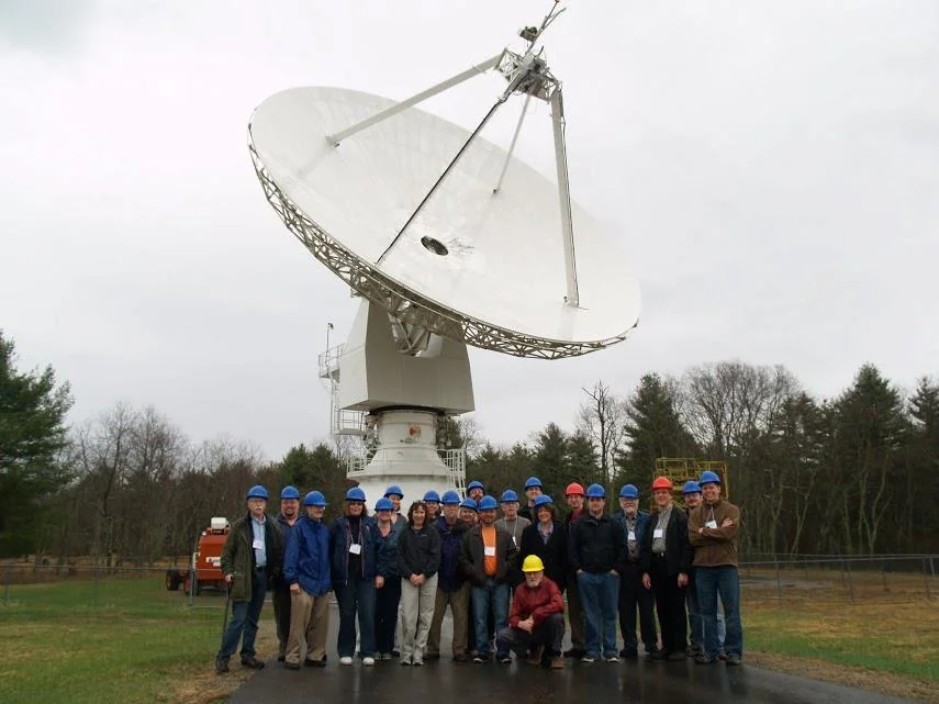
Attendees of the first workshop for science and education with Skynet.
Regarding student, as well as public, use, the 20-meter represents a significant opportunity for radio astronomy. Small optical telescopes can be found on many, if not most, college campuses. But small radio telescopes are significantly more expensive to build, operate, and maintain, and consequently are generally found only in remote locations that make the most sense for professional use. Consequently, most people—including most students of astronomy—never experience radio telescopes, let alone use them. However, under the control of Skynet, the 20-meter is not only more accessible to more professionals, it is already being used by thousands of students per year, of all ages, as well as by the public.
New Single-Dish Radio Telescope Image-Processing Algorithms
We are working on a two-paper series in which we present new, more powerful, single-dish radio telescope image-processing algorithms.
Our algorithms significantly leverage a new outlier rejection method, called Robust Chauvenet Rejection (RCR). Traditionally, outlier rejection methods are a trade-off between robustness and precision. For example, the mode is a measure of central tendency that is very robust against contamination by outliers, but it is much less precise than, say, the median or the mean. The mean on the other hand is a very precise measure of central tendency, but at the same time is very prone to being inaccurate if applied to an outlier-contaminated sample. RCR applies decreasingly robust and increasingly precise outlier-rejection methods sequentially, achieving both robustness and precision, even in the face of almost-complete sample contamination. Potential applications are numerous, spanning virtually all quantitative disciplines. However, we have chosen single-dish mapping as its first in-depth application (see also Trotter et al. 2017, in which we use it to better combine gain-calibrated measurements taken at different times.)

Left: Raw map of Virgo A (top), 3C 270 (center right), and 3C 273 (bottom), acquired with the 20-meter in L band, using a 1/10-beamwidth horizontal raster. Left and right linear polarization channels have been summed, partially symmetrizing the beam pattern. All three signal contaminants are demonstrated: (1) en-route drift, the low-level variations along the horizontal scans, (2) RFI, both long-duration, during the scan that passes through 3C 273, and short-duration, near Virgo A, and (3) elevation-dependent signal, toward the upper right, which was only ≈11º above the horizon. Middle: After background subtraction, with a 7-beamwidth scales (the map is 24 beamwidths across). Hyperbolic-arcsine scaling is used to emphasize fainter structures. Right: After RFI subtraction, with a 0.9-beamwidth scale. RFI, both long-duration intersecting 3C 273 and short-duration near Virgo A, as well as en-route drift across the entire image, are successfully eliminated. Locally modeled surface haa been applied for visualization, with a minimum weighting scale of 2/3 beamwidths.
The focus of Paper I is contaminant-cleaning, mapping, and photometering small-scale astronomical structures, such as point sources, or moderately extended sources. In Paper I:
1. We use RCR to improve gain calibration, making this procedure insensitive to contamination by radio-frequency interference (RFI; as long as the contamination is not complete, or nearly complete), to catching the noise diode in transition, and to the background level ramping up or down (linearly), for whatever reason, during the calibration.

Top left: (Time-delay corrected) raw maps of Andromeda, acquired with GBO’s 40-foot diameter radio telescope in L band, using a maximum slew speed nodding pattern. Instrumental signal drift dominates each map. Bottom left: Data from the top row background-subtracted, with a 5-beamwidth scale (larger than the minimum recommended scale, given the size of the source). Similar maps are extracted, despite the large systematics. Right: After appending and then jointly RFI-subtracting, with a 0.7-beamwidth scale. Locally modeled surface has been applied for visualization, with a minimum weighting scale of 1/3 beamwidths.
2. We again use RCR to measure the noise level of the data, in this case from point to point along the scans of the telescope’s mapping pattern, also allowing this level to ramp up or down (again, linearly) over the course of the observation. We then use this noise model to background-subtract the data along each scan, without significantly biasing these data high or low. We do this by modeling the background locally, within a user-defined scale, instead of globally and hence less flexibly (as, e.g., basket-weaving approaches do). This significantly reduces, if not outright eliminates, most signal contaminants: en-route drift (also known as the scanning effect), long-duration (but not short-duration) RFI, astronomical signal on larger scales, and elevation-dependent signal. Furthermore, this procedure requires only a single mapping (also unlike basket-weaving approaches).
3. We use RCR to correct for any time delay between signal measurements and coordinate measurements. This method is robust against contamination by short-duration RFI and residual long-duration RFI. (In general, this procedure requires that the telescope’s slew speed remain nearly constant throughout the mapping, or at least during its scans if not between them, though we do offer a modification such that it can also be applied to variable-speed, daisy mapping patterns, centered on a source.)

Left: Background-subtracted mapping of, from right to left, 3C 84, NRAO 1560/1650, 3C 111, 3C 123, 3C 139.1, and 3C 147, as well as fainter sources, acquired with the 40-foot in L band, using a maximum slew speed nodding pattern. The data are heavily contaminated by linearly polarized, broadband RFI, affecting only one of the receiver’s two polarization channels. Middle: Data from the left panel time-delay corrected and RFI-subtracted, with a 0.7-beamwidth scale. Right: Identically processed data from the receiver’s other, relatively uncontaminated polarization channel, for comparison. The RFI-subtraction algorithm is not perfect, but performs very well given the original, extreme level of contamination.
4. We again measure the noise level of the data, but this time from point to point across the scans, again allowing this level to ramp up or down (again, linearly) over the course of the observation. We then use this noise model to RFI-subtract the data, again without significantly biasing these data high or low. We do this by modeling the RFI-subtracted signal locally, over a user-defined scale; structures that are smaller than this scale, either along or across scans, are eliminated, including short-duration RFI, residual long-duration RFI, residual en-route drift, etc. This scale can be set to preserve only diffraction-limited point sources and larger structures, or it can be halved to additionally preserve Airy rings, which are visible around the brightest sources. Furthermore, this procedure can be applied to multiple observations simultaneously, in which case even smaller scales can be used (better preserving noise-level signal, and hence faint, low-S/N sources).

Top: On-the-fly mapping patterns: horizontal raster (left), nodding (middle), and daisy (right). Bottom: Weighted modeling of 20-meter data from the horizontal raster mapping of Virgo A from above, at two representative points. Modeled surfaces span two beamwidths, but are most strongly weighted to fit the data over only the central, typically, 1/3 – 2/3 beamwidths. Only the central point (red) is retained.
5. To interpolate between signal measurements, we introduce an algorithm for modeling the data, over a user-defined weighting scale (though the algorithm can increase this scale, from place to place in the image, if more data are required for a stable, local solution). Advantages of this approach are: (1) It does not blur the image beyond its native, diffraction-limited resolution; (2) It may be applied at any stage in our contaminant-cleaning algorithm, for visualization of each step, if desired; and (3) Any pixel density may be selected. This stands in contrast to existing algorithms, which use weighted averaging to regrid the data: (1) This does blur the image beyond its native resolution, often significantly; (2) It is usually done before contaminant cleaning takes place, because existing contaminant-cleaning algorithms – unlike ours – require gridded data; and (3) The pixel density is then necessarily limited to what these contaminant-cleaning algorithms can handle, computationally.
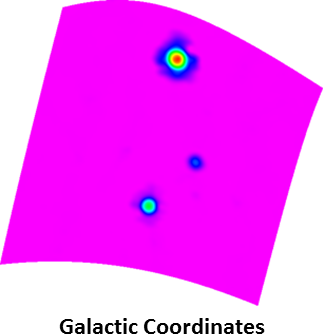
Bottom right: Mapping of Virgo A from above processed in Galactic coordinates, vs. its original, equatorial coordinate system. This field is at high Galactic latitude, and consequently serves as a good example of the equal-areas and equal-distances properties of our sinusoidal projection. Equal areas means that sources cover the same number of pixels, and consequently should yield approximately the same photometry: The three sources in this map yields the same photometry as in the bottom-left panel to within 3%, despite the greater (diagonal) distortion that these sources can experience at high Galactic latitudes. Equal distances refers to distances along horizontal lines, as well as along the central vertical axis, being distortion-free.
Furthermore, since our surface-modeling algorithm does not require gridded data, images can be produced in any coordinate system, regardless of how the mapping pattern was designed. And since our surface-modeling algorithm does not assume any coordinate system-based symmetries, it works equally well with asymmetric structures. In addition to the final image, we produce a path map, a scale map, a weight map, and a correlation map, the latter three of which are important when performing photometry on the final image.
6. Lastly, we introduce an aperture-photometry algorithm for use with these images. In particular, we introduce a semi-empirical method for estimating photometric error bars from a single image, which is non-trivial given the non-independence of pixel values in these reconstructed images (unlike in, e.g., CCD images, where each pixel value is independent, and consequently the statistics are simpler). We also provide an empirical correction for low-S/N photometry, which can be underestimated in these reconstructed images.
In Paper II, we expand on the algorithm that we presented in Paper I (1) to additionally contaminant-clean and map larger-scale astronomical structures, and (2) to do the same for spectral (as opposed to just continuum) observations. We also present an X-band survey of the Galactic plane, from -5º < l < 95º, the data for which we collected with the 20-meter, to showcase, and further test, many of the techniques that we developed in both of these papers.
Radio Afterglow
Once we have completed Paper II, and the optical components of Afterglow 2.0, we will begin to integrate these (and other) new, single-dish radio telescope processing capabilities into Afterglow, making both collection and analysis of single-dish radio data straightforward for both professional and student users.